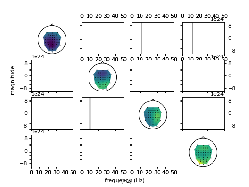
misc example code: statistics.py

(Source code, png, hires.png, pdf)

"""
This example shows how to create surrogate connectivity to determine if
connectivity is statistically significant.
"""

import numpy as np

import scot
import numpy as np

# The data set contains a continuous 45 channel EEG recording of a motor
# imagery experiment. The data was preprocessed to reduce eye movement
# artifacts and resampled to a sampling rate of 100 Hz. With a visual cue, the
# subject was instructed to perform either hand or foot motor imagery. The
# trigger time points of the cues are stored in 'triggers', and 'classes'
# contains the class labels. Duration of the motor imagery period was
# approximately six seconds.
from scot.datasets import fetch


midata = fetch("mi")[0]

raweeg = midata["eeg"]
triggers = midata["triggers"]
classes = midata["labels"]
fs = midata["fs"]
locs = midata["locations"]


# Set random seed for repeatable results
np.random.seed(42)


# Prepare data
#
# Here we cut out segments from 3s to 4s after each trigger. This is right in
# the middle of the motor imagery period.
data = scot.datatools.cut_segments(raweeg, triggers, 3 * fs, 4 * fs)


# Set up analysis object
#
# We choose a VAR model order of 35, and reduction to 4 components.
ws = scot.Workspace({'model_order': 35}, reducedim=4, fs=fs, locations=locs)

fig = None

# Perform MVARICA and plot components
ws.set_data(data, classes)
ws.do_mvarica(varfit='class')

p = ws.var_.test_whiteness(50)
print('Whiteness:', p)

fig = ws.plot_connectivity_topos(fig=fig)

p, s, _ = ws.compare_conditions(['hand'], ['foot'], 'ffDTF', repeats=100,
                                plot=fig)

print(p)
ws.show_plots()