# Released under The MIT License (MIT)
# http://opensource.org/licenses/MIT
# Copyright (c) 2013-2015 SCoT Development Team
"""
This example shows how to decompose EEG signals into source activations with
MVARICA, and visualize time varying connectivity.
"""
import numpy as np
import scot
# The data set contains a continuous 45 channel EEG recording of a motor
# imagery experiment. The data was preprocessed to reduce eye movement
# artifacts and resampled to a sampling rate of 100 Hz. With a visual cue, the
# subject was instructed to perform either hand or foot motor imagery. The
# trigger time points of the cues are stored in 'triggers', and 'classes'
# contains the class labels. Duration of the motor imagery period was
# approximately six seconds.
from scot.datasets import fetch
midata = fetch("mi")[0]
raweeg = midata["eeg"]
triggers = midata["triggers"]
classes = midata["labels"]
fs = midata["fs"]
locs = midata["locations"]
# Set random seed for repeatable results
np.random.seed(42)
# Set up analysis object
#
# We simply choose a VAR model order of 35, and reduction to 4 components.
ws = scot.Workspace({'model_order': 40}, reducedim=4, fs=fs, locations=locs)
# Prepare data
#
# Here we cut out segments from 3s to 4s after each trigger. This is right in
# the middle of the motor imagery period.
data = scot.datatools.cut_segments(raweeg, triggers, 3 * fs, 4 * fs)
# Perform CSPVARICA
ws.set_data(data, classes)
ws.do_cspvarica()
p = ws.var_.test_whiteness(50)
print('Whiteness:', p)
# Prepare data
#
# Here we cut out segments from -2s to 8s around each trigger. This covers the
# whole trial
data = scot.datatools.cut_segments(raweeg, triggers, -2 * fs, 8 * fs)
# Configure plotting options
ws.plot_f_range = [0, 30] # only show 0-30 Hz
ws.plot_diagonal = 'topo' # put topo plots on the diagonal
ws.plot_outside_topo = False # no topo plots above and to the left
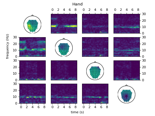
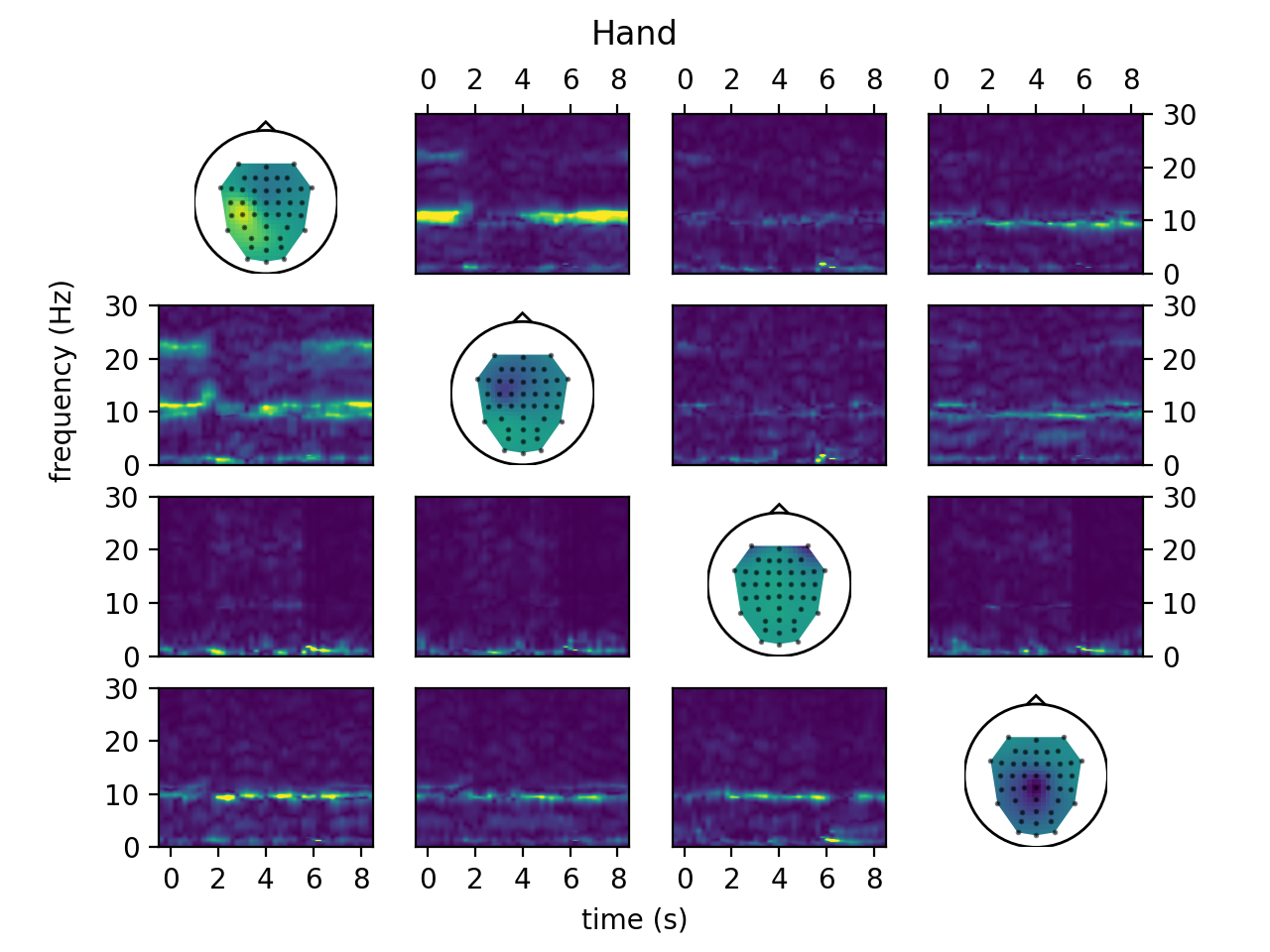
# Connectivity analysis
#
# Extract the full frequency directed transfer function (ffDTF) from the
# activations of each class and plot them.
ws.set_data(data, classes, time_offset=-1)
fig = ws.plot_connectivity_topos()
ws.set_used_labels(['hand'])
ws.get_tf_connectivity('ffDTF', 1 * fs, int(0.2 * fs), plot=fig,
crange=[0, 30])
fig.suptitle('Hand')
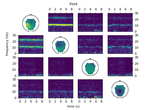
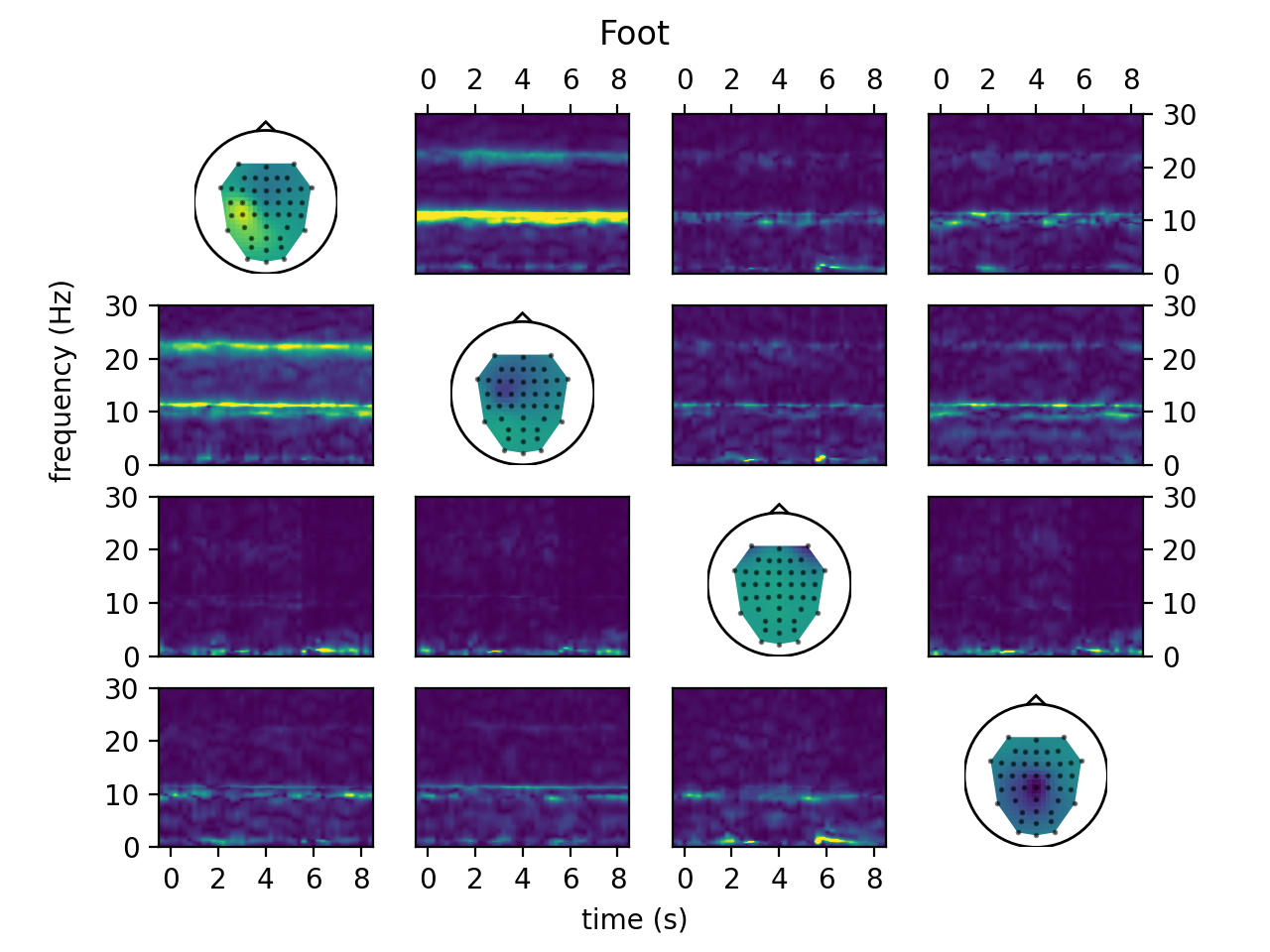
fig = ws.plot_connectivity_topos()
ws.set_used_labels(['foot'])
ws.get_tf_connectivity('ffDTF', 1 * fs, int(0.2 * fs), plot=fig,
crange=[0, 30])
fig.suptitle('Foot')
ws.show_plots()

