"""
This example shows how to decompose EEG signals into source activations with
CSPVARICA and visualize connectivity.
"""
import numpy as np
import matplotlib.pyplot as plt
import scot
from scot.utils import cuthill_mckee
from scot.eegtopo.topoplot import Topoplot
from scot import plotting
# The data set contains a continuous 45 channel EEG recording of a motor
# imagery experiment. The data was preprocessed to reduce eye movement
# artifacts and resampled to a sampling rate of 100 Hz. With a visual cue, the
# subject was instructed to perform either hand or foot motor imagery. The
# trigger time points of the cues are stored in 'triggers', and 'classes'
# contains the class labels. Duration of the motor imagery period was
# approximately six seconds.
from scot.datasets import fetch
midata = fetch("mi")[0]
raweeg = midata["eeg"]
triggers = midata["triggers"]
classes = midata["labels"]
fs = midata["fs"]
locs = midata["locations"]
# Set random seed for repeatable results
np.random.seed(42)
# Prepare data
#
# Here we cut out segments from 2s to 5s after each trigger. This is right in
# the middle of the motor imagery period.
data = scot.datatools.cut_segments(raweeg, triggers, 2 * fs, 5 * fs)
# Set up analysis object
#
# We simply choose a VAR model order of 30, and reduction to 15 components.
ws = scot.Workspace({'model_order': 30}, reducedim=15, fs=fs, locations=locs)
# Perform CSPVARICA
ws.set_data(data, classes)
ws.do_cspvarica()
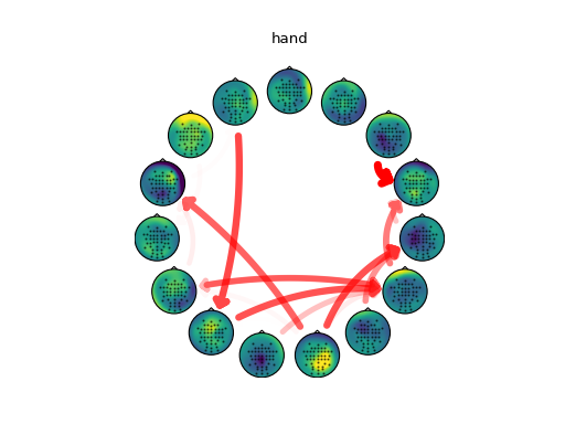
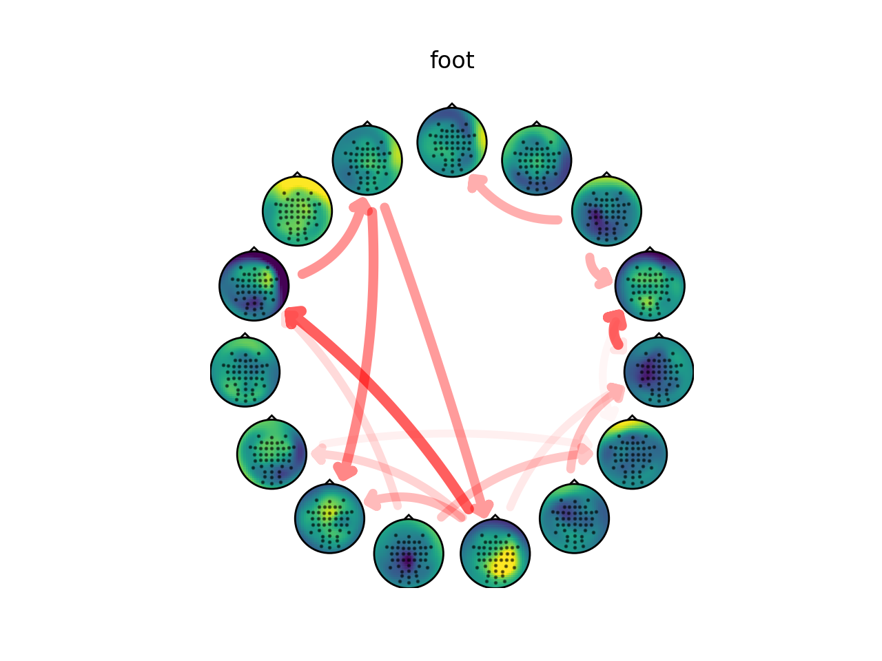
# Connectivity analysis
#
# Extract the full frequency directed transfer function (ffDTF) from the
# activations of each class and calculate the average value over the alpha band
# (8-12 Hz).
freq = np.linspace(0, fs, ws.nfft_)
alpha, beta = {}, {}
for c in np.unique(classes):
ws.set_used_labels([c])
ws.fit_var()
con = ws.get_connectivity('ffDTF')
alpha[c] = np.mean(con[:, :, np.logical_and(8 < freq, freq < 12)], axis=2)
# Prepare topography plots
topo = Topoplot()
topo.set_locations(locs)
mixmaps = plotting.prepare_topoplots(topo, ws.mixing_)
# Force diagonal (self-connectivity) to 0
np.fill_diagonal(alpha['hand'], 0)
np.fill_diagonal(alpha['foot'], 0)
order = None
for cls in ['hand', 'foot']:
np.fill_diagonal(alpha[cls], 0)
w = alpha[cls]
m = alpha[cls] > 4
# use same ordering of components for each class
if not order:
order = cuthill_mckee(m)
# fixed color, but alpha varies with connectivity strength
r = np.ones(w.shape)
g = np.zeros(w.shape)
b = np.zeros(w.shape)
a = (alpha[cls]-4) / max(np.max(alpha['hand']-4), np.max(alpha['foot']-4))
c = np.dstack([r, g, b, a])
plotting.plot_circular(colors=c, widths=w, mask=m, topo=topo,
topomaps=mixmaps, order=order)
plt.title(cls)
plotting.show_plots()

