scot package¶

Subpackages¶

Submodules¶

scot.backend_builtin module¶

Use internally implemented functions as backend.

scot.backend_builtin.generate()¶

scot.backend_mne module¶

Use mne-python routines as backend.

scot.backend_mne.generate()¶

scot.backend_sklearn module¶

Use scikit-learn routines as backend.

scot.backend_sklearn.generate()¶

scot.backendmanager module¶

class scot.backendmanager.BackendManager¶

Bases: object

activate(name)¶

get_backend(name)¶

items()¶

names()¶

register(name, activation_function)¶

scot.config module¶

scot.config.load_configuration()¶

scot.connectivity module¶

Connectivity analysis

class scot.connectivity.Connectivity(b, c=None, nfft=512)¶

Bases: object

Calculation of connectivity measures.

This class calculates various spectral connectivity measures from a vector autoregressive (VAR) model.

Parameters:

barray, shape (n_channels, n_channels * model_order): VAR model coefficients. See On the arrangement of VAR model coefficients for details about the arrangement of coefficients.
carray, shape (n_channels, n_channels), optional: Covariance matrix of the driving noise process. Identity matrix is used if set to None (default).
nfftint, optional: Number of frequency bins to calculate. Note that these points cover the range between 0 and half the sampling rate.

Notes

Connectivity measures are returned by member functions that take no arguments and return a matrix of shape (m, m, nfft). The first dimension is the sink, the second dimension is the source, and the third dimension is the frequency.

An overview of most supported measures can be found in [1].

References

[1]

M. Billinger, C. Brunner, G. R. Müller-Putz. Single-trial connectivity estimation for classification of motor imagery data. J. Neural Eng. 10, 2013.

Methods

:func:`A`	Spectral representation of the VAR coefficients.
:func:`H`	Transfer function (turns the innovation process into the VAR process).
:func:`S`	Cross-spectral density.
:func:`logS`	Logarithm of the cross-spectral density (S).
:func:`G`	Inverse cross-spectral density.
:func:`logG`	Logarithm of the inverse cross-spectral density.
:func:`PHI`	Phase angle.
:func:`COH`	Coherence.
:func:`pCOH`	Partial coherence.
:func:`PDC`	Partial directed coherence.
:func:`ffPDC`	Full frequency partial directed coherence.
:func:`PDCF`	PDC factor.
:func:`GPDC`	Generalized partial directed coherence.
:func:`DTF`	Directed transfer function.
:func:`ffDTF`	Full frequency directed transfer function.
:func:`dDTF`	Direct directed transfer function.
:func:`GDTF`	Generalized directed transfer function.

A()¶: Spectral VAR coefficients.

\[\mathbf{A}(f) = \mathbf{I} - \sum_{k=1}^{p} \mathbf{a}^{(k)} \mathrm{e}^{-2\pi f}\]

COH()¶

Coherence.

\[\begin{split}\mathrm{COH}_{ij}(f) = \\frac{S_{ij}(f)} {\sqrt{S_{ii}(f) S_{jj}(f)}}\end{split}\]

References

P. L. Nunez, R. Srinivasan, A. F. Westdorp, R. S. Wijesinghe, D. M. Tucker, R. B. Silverstein, P. J. Cadusch. EEG coherency I: statistics, reference electrode, volume conduction, Laplacians, cortical imaging, and interpretation at multiple scales. Electroenceph. Clin. Neurophysiol. 103(5): 499-515, 1997.

Cinv()¶: Inverse of the noise covariance.

DTF()¶

Directed transfer function.

\[\begin{split}\mathrm{DTF}_{ij}(f) = \\frac{H_{ij}(f)} {\sqrt{H_{i:}(f) H_{i:}'(f)}}\end{split}\]

References

M. J. Kaminski, K. J. Blinowska. A new method of the description of the information flow in the brain structures. Biol. Cybernetics 65(3): 203-210, 1991.

G()¶: Inverse cross-spectral density.

\[\mathbf{G}(f) = \mathbf{A}(f) \mathbf{C}^{-1} \mathbf{A}'(f)\]

GDTF()¶

Generalized directed transfer function.

\[\begin{split}\mathrm{GPDC}_{ij}(f) = \\frac{\sigma_j |H_{ij}(f)|} {\sqrt{H_{i:}(f) \mathrm{diag}(\mathbf{C}) H_{i:}'(f)}}\end{split}\]

References

L. Faes, S. Erla, G. Nollo. Measuring connectivity in linear multivariate processes: definitions, interpretation, and practical analysis. Comput. Math. Meth. Med. 2012: 140513, 2012.

GPDC()¶

Generalized partial directed coherence.

\[\begin{split}\mathrm{GPDC}_{ij}(f) = \\frac{|A_{ij}(f)|}\end{split}\]

{sigma_i sqrt{A_{:j}’(f) mathrm{diag}(mathbf{C})^{-1} A_{:j}(f)}}

References

L. Faes, S. Erla, G. Nollo. Measuring connectivity in linear multivariate processes: definitions, interpretation, and practical analysis. Comput. Math. Meth. Med. 2012: 140513, 2012.

H()¶: VAR transfer function.

\[\mathbf{H}(f) = \mathbf{A}(f)^{-1}\]

PDC()¶

Partial directed coherence.

\[\begin{split}\mathrm{PDC}_{ij}(f) = \\frac{A_{ij}(f)} {\sqrt{A_{:j}'(f) A_{:j}(f)}}\end{split}\]

References

L. A. Baccalá, K. Sameshima. Partial directed coherence: a new concept in neural structure determination. Biol. Cybernetics 84(6): 463-474, 2001.

PDCF()¶

Partial directed coherence factor.

\[\mathrm{PDCF}_{ij}(f) =\]

\frac{A_{ij}(f)}{sqrt{A_{:j}’(f) mathbf{C}^{-1} A_{:j}(f)}}

References

L. A. Baccalá, K. Sameshima. Partial directed coherence: a new concept in neural structure determination. Biol. Cybernetics 84(6): 463-474, 2001.

PHI()¶

Phase angle.

Phase angle of complex S().

S()¶: Cross-spectral density.

\[\mathbf{S}(f) = \mathbf{H}(f) \mathbf{C} \mathbf{H}'(f)\]

absS()¶: Absolute cross-spectral density.

\[\mathrm{absS}(f) = | \mathbf{S}(f) |\]

dDTF()¶

Direct directed transfer function.

\[\mathrm{dDTF}_{ij}(f) = |\mathrm{pCOH}_{ij}(f)| \mathrm{ffDTF}_{ij}(f)\]

References

A. Korzeniewska, M. Mańczak, M. Kaminski, K. J. Blinowska, S. Kasicki. Determination of information flow direction among brain structures by a modified directed transfer function (dDTF) method. J. Neurosci. Meth. 125(1-2): 195-207, 2003.

ffDTF()¶

Full frequency directed transfer function.

\[\begin{split}\mathrm{ffDTF}_{ij}(f) = \\frac{H_{ij}(f)}{\sqrt{\sum_f H_{i:}(f) H_{i:}'(f)}}\end{split}\]

References

ffPDC()¶: Full frequency partial directed coherence.

\[\begin{split}\mathrm{ffPDC}_{ij}(f) = \\frac{A_{ij}(f)}{\sqrt{\sum_f A_{:j}'(f) A_{:j}(f)}}\end{split}\]

logG()¶: Logarithmic inverse cross-spectral density.

\[\mathrm{logG}(f) = \log | \mathbf{G}(f) |\]

logS()¶: Logarithmic cross-spectral density.

\[\mathrm{logS}(f) = \log | \mathbf{S}(f) |\]

pCOH()¶

Partial coherence.

\[\begin{split}\mathrm{pCOH}_{ij}(f) = \\frac{G_{ij}(f)} {\sqrt{G_{ii}(f) G_{jj}(f)}}\end{split}\]

References

P. J. Franaszczuk, K. J. Blinowska, M. Kowalczyk. The application of parametric multichannel spectral estimates in the study of electrical brain activity. Biol. Cybernetics 51(4): 239-247, 1985.

sPDC()¶

Squared partial directed coherence.

\[\begin{split}\mathrm{sPDC}_{ij}(f) = \\frac{|A_{ij}(f)|^2} {\mathbf{1}^T | A_{:j}(f) |^2}\end{split}\]

References

L. Astolfi, F. Cincotti, D. Mattia, M. G. Marciani, L. Baccala, F. D. Fallani, S. Salinari, M. Ursino, M. Zavaglia, F. Babiloni. Partial directed coherence: a new concept in neural structure determination. IEEE Trans. Biomed. Eng. 53(9): 1802-1812, 2006.

scot.connectivity.connectivity(measure_names, b, c=None, nfft=512)¶

Calculate connectivity measures.

Parameters:

measure_namesstr or list of str: Name(s) of the connectivity measure(s) to calculate. See Connectivity for supported measures.
barray, shape (n_channels, n_channels * model_order): VAR model coefficients. See On the arrangement of VAR model coefficients for details about the arrangement of coefficients.
carray, shape (n_channels, n_channels), optional: Covariance matrix of the driving noise process. Identity matrix is used if set to None (default).
nfftint, optional: Number of frequency bins to calculate. Note that these points cover the range between 0 and half the sampling rate.

Returns:

resultarray, shape (n_channels, n_channels, nfft): An array of shape (m, m, nfft) is returned if measures is a string. If measures is a list of strings, a dictionary is returned, where each key is the name of the measure, and the corresponding values are arrays of shape (m, m, nfft).

Notes

When using this function, it is more efficient to get several measures at once than calling the function multiple times.

Examples

>>> c = connectivity(['DTF', 'PDC'], [[0.3, 0.6], [0.0, 0.9]])

scot.connectivity_statistics module¶

Routines for statistical evaluation of connectivity.

scot.connectivity_statistics.bootstrap_connectivity(measures, data, var, nfft=512, repeats=100, num_samples=None, n_jobs=1, verbose=0, random_state=None)¶

Calculate bootstrap estimates of connectivity.

To obtain a bootstrap estimate trials are sampled randomly with replacement from the data set.

Note

Parameter var will be modified by the function. Treat as

undefined after the function returns.

Parameters:

measuresstr or list of str: Name(s) of the connectivity measure(s) to calculate. See Connectivity for supported measures.
dataarray, shape (trials, channels, samples): Time series data (multiple trials).
varVARBase-like object: Instance of a VAR model.
nfftint, optional: Number of frequency bins to calculate. Note that these points cover the range between 0 and half the sampling rate.
repeatsint, optional: Number of bootstrap estimates to take.
num_samplesint, optional: Number of samples to take for each bootstrap estimates. Defaults to the same number of trials as present in the data.
n_jobsint, optional: n_jobs : int | None, optional Number of jobs to run in parallel. If set to None, joblib is not used at all. See joblib.Parallel for details.
verboseint, optional: Verbosity level passed to joblib.

Returns:

measurearray, shape (repeats, n_channels, n_channels, nfft): Values of the connectivity measure for each bootstrap estimate. If measure_names is a list of strings a dictionary is returned, where each key is the name of the measure, and the corresponding values are arrays of shape (repeats, n_channels, n_channels, nfft).

scot.connectivity_statistics.convert_output_(output, measures)¶

scot.connectivity_statistics.jackknife_connectivity(measures, data, var, nfft=512, leaveout=1, n_jobs=1, verbose=0)¶

Calculate jackknife estimates of connectivity.

For each jackknife estimate a block of trials is left out. This is repeated until each trial was left out exactly once. The number of estimates depends on the number of trials and the value of leaveout. It is calculated by repeats = n_trials // leaveout.

Note

Parameter var will be modified by the function. Treat as

undefined after the function returns.

Parameters:

measuresstr or list of str: Name(s) of the connectivity measure(s) to calculate. See Connectivity for supported measures.
dataarray, shape (trials, channels, samples): Time series data (multiple trials).
varVARBase-like object: Instance of a VAR model.
nfftint, optional: Number of frequency bins to calculate. Note that these points cover the range between 0 and half the sampling rate.
leaveoutint, optional: Number of trials to leave out in each estimate.
n_jobsint | None, optional: Number of jobs to run in parallel. If set to None, joblib is not used at all. See joblib.Parallel for details.
verboseint, optional: Verbosity level passed to joblib.

Returns:

resultarray, shape (repeats, n_channels, n_channels, nfft): Values of the connectivity measure for each surrogate. If measure_names is a list of strings a dictionary is returned, where each key is the name of the measure, and the corresponding values are arrays of shape (repeats, n_channels, n_channels, nfft).

scot.connectivity_statistics.significance_fdr(p, alpha)¶

Calculate significance by controlling for the false discovery rate.

This function determines which of the p-values in p can be considered significant. Correction for multiple comparisons is performed by controlling the false discovery rate (FDR). The FDR is the maximum fraction of p-values that are wrongly considered significant [1].

Parameters:

parray, shape (channels, channels, nfft): p-values.
alphafloat: Maximum false discovery rate.

Returns:

sarray, dtype=bool, shape (channels, channels, nfft): Significance of each p-value.

References

[1]

Y. Benjamini, Y. Hochberg. Controlling the false discovery rate: a practical and powerful approach to multiple testing. J. Royal Stat. Soc. Series B 57(1): 289-300, 1995.

scot.connectivity_statistics.surrogate_connectivity(measure_names, data, var, nfft=512, repeats=100, n_jobs=1, verbose=0, random_state=None)¶

Calculate surrogate connectivity for a multivariate time series by phase randomization [1].

Note

Parameter var will be modified by the function. Treat as

undefined after the function returns.

Parameters:

measuresstr or list of str: Name(s) of the connectivity measure(s) to calculate. See Connectivity for supported measures.
dataarray, shape (trials, channels, samples) or (channels, samples): Time series data (2D or 3D for multiple trials)
varVARBase-like object: Instance of a VAR model.
nfftint, optional: Number of frequency bins to calculate. Note that these points cover the range between 0 and half the sampling rate.
repeatsint, optional: Number of surrogate samples to take.
n_jobsint | None, optional: Number of jobs to run in parallel. If set to None, joblib is not used at all. See joblib.Parallel for details.
verboseint, optional: Verbosity level passed to joblib.

Returns:

resultarray, shape (repeats, n_channels, n_channels, nfft): Values of the connectivity measure for each surrogate. If measure_names is a list of strings a dictionary is returned, where each key is the name of the measure, and the corresponding values are arrays of shape (repeats, n_channels, n_channels, nfft).

[1]

J. Theiler et al. Testing for nonlinearity in time series: the method of surrogate data. Physica D, 58: 77-94, 1992.

scot.csp module¶

Common spatial patterns (CSP) implementation.

scot.csp.csp(x, cl, numcomp=None)¶

Calculate common spatial patterns (CSP).

Parameters:

xarray, shape (trials, channels, samples) or (channels, samples): EEG data set.
cllist of valid dict keys: Class labels associated with each trial. Currently, only two classes are supported.
numcompint, optional: Number of patterns to keep after applying CSP. If numcomp is greater than channels or None, all patterns are returned.

Returns:

warray, shape (channels, components): CSP weight matrix.
varray, shape (components, channels): CSP projection matrix.

scot.datasets module¶

exception scot.datasets.MD5MismatchError¶: Bases: Exception

scot.datasets.convert(dataset, mat)¶

scot.datasets.fetch(dataset='mi', datadir='/home/martin/scot_data')¶

Fetch example dataset.

If the requested dataset is not found in the location specified by datadir, the function attempts to download it.

Parameters:

datasetstr: Which dataset to load. Currently only ‘mi’ is supported.
datadirstr: Path to the storage location of example datasets. Datasets are downloaded to this location if they cannot be found. If the directory does not exist it is created.

Returns:

datalist of dicts: The data set is stored in a list, where each list element corresponds to data from one subject. Each list element is a dictionary with the following keys: - “eeg” … EEG signals - “triggers” … Trigger latencies - “labels” … Class labels - “fs” … Sample rate - “locations” … Channel locations

scot.datatools module¶

Summary¶

Tools for basic data manipulation.

scot.datatools.acm(x, l)¶

Compute autocovariance matrix at lag l.

This function calculates the autocovariance matrix of x at lag l.

Parameters:

xarray, shape (n_trials, n_channels, n_samples): Signal data (2D or 3D for multiple trials)
lint: Lag

Returns:

cndarray, shape = [nchannels, n_channels]: Autocovariance matrix of x at lag l.

scot.datatools.atleast_3d(x)¶

scot.datatools.cat_trials(x3d)¶

Concatenate trials along time axis.

Parameters:

x3darray, shape (t, m, n): Segmented input data with t trials, m signals, and n samples.

Returns:

x2darray, shape (m, t * n): Trials are concatenated along the second axis.

See also

cut_segments: Cut segments from continuous data.

Examples

>>> x = np.random.randn(6, 4, 150)
>>> y = cat_trials(x)
>>> y.shape
(4, 900)

scot.datatools.cut_segments(x2d, tr, start, stop)¶

Cut continuous signal into segments.

Parameters:

x2darray, shape (m, n): Input data with m signals and n samples.
trlist of int: Trigger positions.
startint: Window start (offset relative to trigger).
stopint: Window end (offset relative to trigger).

Returns:

x3darray, shape (len(tr), m, stop-start): Segments cut from data. Individual segments are stacked along the first dimension.

See also

cat_trials: Concatenate segments.

Examples

>>> data = np.random.randn(5, 1000)  # 5 channels, 1000 samples
>>> tr = [750, 500, 250]  # three segments
>>> x3d = cut_segments(data, tr, 50, 100)  # each segment is 50 samples
>>> x3d.shape
(3, 5, 50)

scot.datatools.dot_special(x2d, x3d)¶

Segment-wise dot product.

This function calculates the dot product of x2d with each trial of x3d.

Parameters:

x2darray, shape (p, m): Input argument.
x3darray, shape (t, m, n): Segmented input data with t trials, m signals, and n samples. The dot product with x2d is calculated for each trial.

Returns:

outarray, shape (t, p, n): Dot product of x2d with each trial of x3d.

Examples

>>> x = np.random.randn(6, 40, 150)
>>> a = np.ones((7, 40))
>>> y = dot_special(a, x)
>>> y.shape
(6, 7, 150)

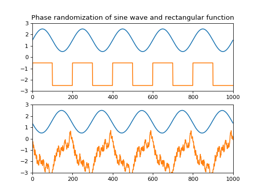
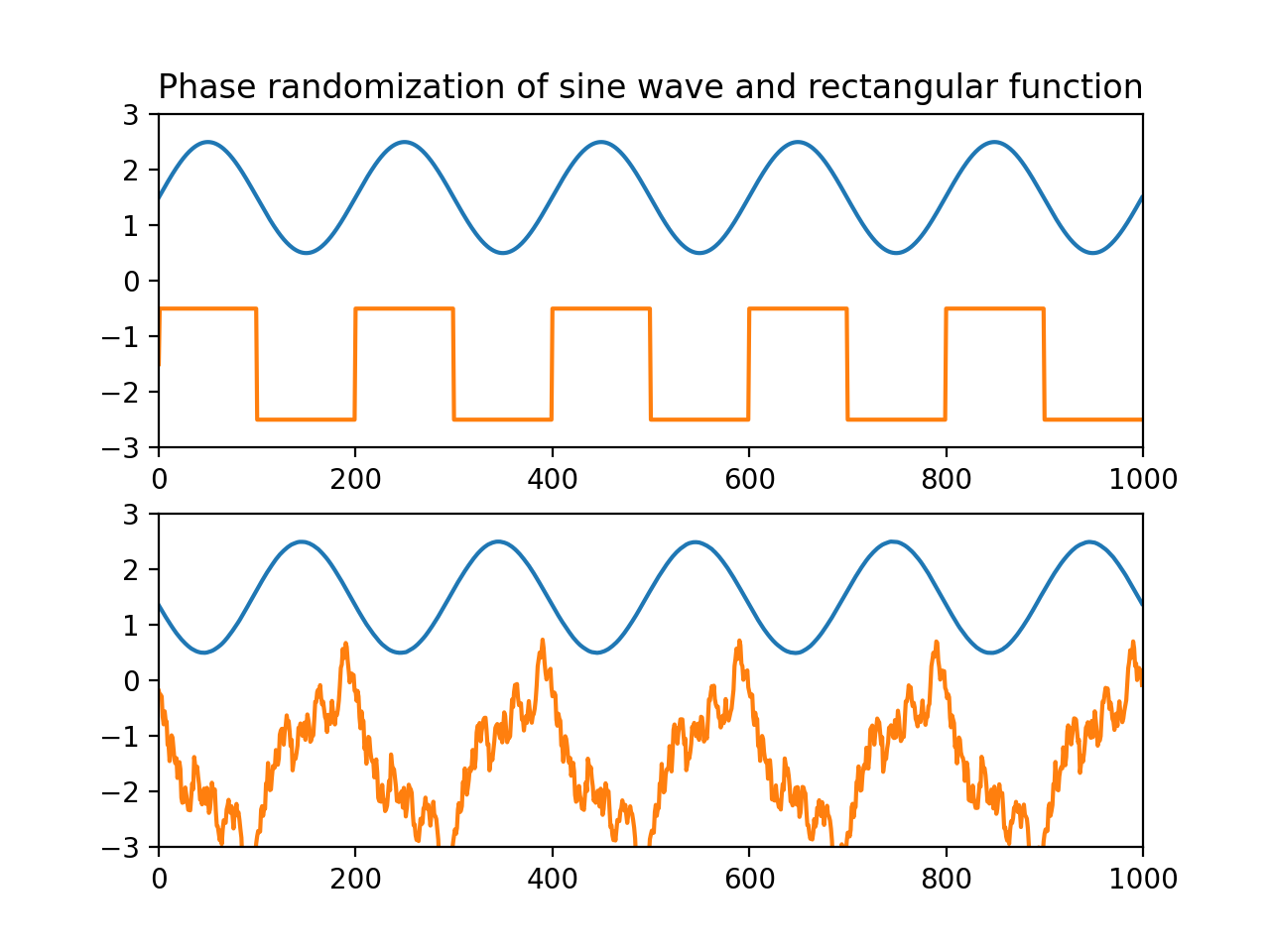
scot.datatools.randomize_phase(data, random_state=None)¶

Phase randomization.

This function randomizes the spectral phase of the input data along the last dimension.

Parameters:

dataarray: Input array.

Returns:

outarray: Array of same shape as data.

Notes

The algorithm randomizes the phase component of the input’s complex Fourier transform.

Examples

from pylab import *
from scot.datatools import randomize_phase
np.random.seed(1234)
s = np.sin(np.linspace(0,10*np.pi,1000))
x = np.vstack([s, np.sign(s)])
y = randomize_phase(x)
subplot(2,1,1)
title('Phase randomization of sine wave and rectangular function')
plot(x.T + [1.5, -1.5]), axis([0,1000,-3,3])
subplot(2,1,2)
plot(y.T + [1.5, -1.5]), axis([0,1000,-3,3])
plt.show()

(Source code, png, hires.png, pdf)

scot.matfiles module¶

Summary¶

Routines for loading and saving Matlab’s .mat files.

scot.matfiles.loadmat(filename)¶: This function should be called instead of direct spio.loadmat as it cures the problem of not properly recovering python dictionaries from mat files. It calls the function check keys to cure all entries which are still mat-objects

scot.ooapi module¶

Summary¶

Object oriented API to SCoT.

Extended Summary¶

The object oriented API provides a the Workspace class, which provides high-level functionality and serves as an example usage of the low-level API.

class scot.ooapi.Workspace(var, locations=None, reducedim=None, nfft=512, fs=2, backend=None)¶

Bases: object

SCoT Workspace

This class provides high-level functionality for source identification, connectivity estimation, and visualization.

Parameters:

var{VARBase-like object, dict}: Vector autoregressive model (VAR) object that is used for model fitting. This can also be a dictionary that is passed as **kwargs to backend[‘var’]() in order to construct a new VAR model object.
locationsarray_like, optional: 3D Electrode locations. Each row holds the x, y, and z coordinates of an electrode.
reducedim{int, float, ‘no_pca’}, optional: A number of less than 1 in interpreted as the fraction of variance that should remain in the data. All components that describe in total less than 1-reducedim of the variance are removed by the PCA step. An integer number of 1 or greater is interpreted as the number of components to keep after applying the PCA. If set to ‘no_pca’ the PCA step is skipped.
nfftint, optional: Number of frequency bins for connectivity estimation.
backenddict-like, optional: Specify backend to use. When set to None the backend configured in config.backend is used.

Attributes:

`unmixing_`array: Estimated unmixing matrix.
`mixing_`array: Estimated mixing matrix.
`plot_diagonal`str: Configures what is plotted in the diagonal subplots. ‘topo’ (default) plots topoplots on the diagonal, ‘S’ plots the spectral density of each component, and ‘fill’ plots connectivity on the diagonal.
`plot_outside_topo`bool: Whether to place topoplots in the left column and top row.
`plot_f_range`(int, int): Lower and upper frequency limits for plotting. Defaults to [0, fs/2].

compare_conditions(labels1, labels2, measure_name, alpha=0.01, repeats=100, num_samples=None, plot=False, random_state=None)¶

Test for significant difference in connectivity of two sets of class labels.

Connectivity estimates are obtained by bootstrapping. Correction for multiple testing is performed by controlling the false discovery rate (FDR).

Parameters:

labels1, labels2list of class labels: The two sets of class labels to compare. Each set may contain more than one label.
measure_namestr: Name of the connectivity measure to calculate. See Connectivity for supported measures.
alphafloat, optional: Maximum allowed FDR. The ratio of falsely detected significant differences is guaranteed to be less than alpha.
repeatsint, optional: How many bootstrap estimates to take.
num_samplesint, optional: How many samples to take for each bootstrap estimates. Defaults to the same number of trials as present in the data.
plot{False, None, Figure object}, optional: Whether and where to plot the connectivity. If set to False, nothing is plotted. Otherwise set to the Figure object. If set to None, a new figure is created.

Returns:

parray, shape = [n_channels, n_channels, nfft]: Uncorrected p-values.
sarray, dtype=bool, shape = [n_channels, n_channels, nfft]: FDR corrected significance. True means the difference is significant in this location.
figFigure object, optional: Instance of the figure in which was plotted. This is only returned if plot is not False.

do_cspvarica(varfit='ensemble', random_state=None)¶

Perform CSPVARICA

Perform CSPVARICA source decomposition and VAR model fitting.

Parameters:

varfitstring: Determines how to calculate the residuals for source decomposition. ‘ensemble’ (default) fits one model to the whole data set, ‘class’ fits a different model for each class, and ‘trial’ fits a different model for each individual trial.

Returns:

selfWorkspace: The Workspace object.

Raises:

RuntimeError: If the Workspace instance does not contain data.

See also

cspvarica(): CSPVARICA implementation

do_ica(random_state=None)¶

Perform ICA

Perform plain ICA source decomposition.

Returns:

selfWorkspace: The Workspace object.

Raises:

RuntimeError: If the Workspace instance does not contain data.

do_mvarica(varfit='ensemble', random_state=None)¶

Perform MVARICA

Perform MVARICA source decomposition and VAR model fitting.

Parameters:

varfitstring: Determines how to calculate the residuals for source decomposition. ‘ensemble’ (default) fits one model to the whole data set, ‘class’ fits a different model for each class, and ‘trial’ fits a different model for each individual trial.

Returns:

selfWorkspace: The Workspace object.

Raises:

RuntimeError: If the Workspace instance does not contain data.

See also

mvarica(): MVARICA implementation

fit_var()¶

Fit a VAR model to the source activations.

Returns:

selfWorkspace: The Workspace object.

Raises:

RuntimeError: If the Workspace instance does not contain source activations.

get_bootstrap_connectivity(measure_names, repeats=100, num_samples=None, plot=False, random_state=None)¶

Calculate bootstrap estimates of spectral connectivity measures.

Bootstrapping is performed on trial level.

Parameters:

measure_names{str, list of str}: Name(s) of the connectivity measure(s) to calculate. See Connectivity for supported measures.
repeatsint, optional: How many bootstrap estimates to take.
num_samplesint, optional: How many samples to take for each bootstrap estimates. Defaults to the same number of trials as present in the data.

Returns:

measurearray, shape = [repeats, n_channels, n_channels, nfft]: Values of the connectivity measure for each bootstrap estimate. If measure_names is a list of strings a dictionary is returned, where each key is the name of the measure, and the corresponding values are ndarrays of shape [repeats, n_channels, n_channels, nfft].

See also

scot.connectivity_statistics.bootstrap_connectivity(): Calculates bootstrap connectivity

get_connectivity(measure_name, plot=False)¶

Calculate spectral connectivity measure.

Parameters:

measure_namestr: Name of the connectivity measure to calculate. See Connectivity for supported measures.
plot{False, None, Figure object}, optional: Whether and where to plot the connectivity. If set to False, nothing is plotted. Otherwise set to the Figure object. If set to None, a new figure is created.

Returns:

measurearray, shape = [n_channels, n_channels, nfft]: Values of the connectivity measure.
figFigure object: Instance of the figure in which was plotted. This is only returned if plot is not False.

Raises:

RuntimeError: If the Workspace instance does not contain a fitted VAR model.

get_surrogate_connectivity(measure_name, repeats=100, plot=False, random_state=None)¶

Calculate spectral connectivity measure under the assumption of no actual connectivity.

Repeatedly samples connectivity from phase-randomized data. This provides estimates of the connectivity distribution if there was no causal structure in the data.

Parameters:

measure_namestr: Name of the connectivity measure to calculate. See Connectivity for supported measures.
repeatsint, optional: How many surrogate samples to take.

Returns:

measurearray, shape = [repeats, n_channels, n_channels, nfft]: Values of the connectivity measure for each surrogate.

See also

scot.connectivity_statistics.surrogate_connectivity(): Calculates surrogate connectivity

get_tf_connectivity(measure_name, winlen, winstep, plot=False, baseline=None, crange='default')¶

Calculate estimate of time-varying connectivity.

Connectivity is estimated in a sliding window approach on the current data set. The window is stepped n_steps = (n_samples - winlen) // winstep times.

Parameters:

measure_namestr: Name of the connectivity measure to calculate. See Connectivity for supported measures.
winlenint: Length of the sliding window (in samples).
winstepint: Step size for sliding window (in samples).
plot{False, None, Figure object}, optional: Whether and where to plot the connectivity. If set to False, nothing is plotted. Otherwise set to the Figure object. If set to None, a new figure is created.
baseline[int, int] or None: Start and end of the baseline period in samples. The baseline is subtracted from the connectivity. It is computed as the average of all windows that contain start or end, or fall between start and end. If set to None no baseline is subtracted.

Returns:

resultarray, shape = [n_channels, n_channels, nfft, n_steps]: Values of the connectivity measure.
figFigure object, optional: Instance of the figure in which was plotted. This is only returned if plot is not False.

Raises:

RuntimeError: If the Workspace instance does not contain a fitted VAR model.

keep_sources(keep)¶: Keep only the specified sources in the decomposition.

optimize_var()¶

Optimize the VAR model’s hyperparameters (such as regularization).

Returns:

selfWorkspace: The Workspace object.

Raises:

RuntimeError: If the Workspace instance does not contain source activations.

plot_connectivity_surrogate(measure_name, repeats=100, fig=None)¶

Plot spectral connectivity measure under the assumption of no actual connectivity.

Repeatedly samples connectivity from phase-randomized data. This provides estimates of the connectivity distribution if there was no causal structure in the data.

Parameters:

measure_namestr: Name of the connectivity measure to calculate. See Connectivity for supported measures.
repeatsint, optional: How many surrogate samples to take.
fig{None, Figure object}, optional: Where to plot the topos. f set to None, a new figure is created. Otherwise plot into the provided figure object.

Returns:

figFigure object: Instance of the figure in which was plotted.

plot_connectivity_topos(fig=None)¶

Plot scalp projections of the sources.

This function only plots the topos. Use in combination with connectivity plotting.

Parameters:

fig{None, Figure object}, optional: Where to plot the topos. f set to None, a new figure is created. Otherwise plot into the provided figure object.

Returns:

figFigure object: Instance of the figure in which was plotted.

plot_source_topos(common_scale=None)¶

Plot topography of the Source decomposition.

Parameters:

common_scalefloat, optional: If set to None, each topoplot’s color axis is scaled individually. Otherwise specifies the percentile (1-99) of values in all plot. This value is taken as the maximum color scale.

property plotting¶

remove_sources(sources)¶

Remove sources from the decomposition.

This function removes sources from the decomposition. Doing so invalidates currently fitted VAR models and connectivity estimates.

Parameters:

sources{slice, int, array of ints}: Indices of components to remove.

Returns:

selfWorkspace: The Workspace object.

Raises:

RuntimeError: If the Workspace instance does not contain a source decomposition.

set_data(data, cl=None, time_offset=0)¶

Assign data to the workspace.

This function assigns a new data set to the workspace. Doing so invalidates currently fitted VAR models, connectivity estimates, and activations.

Parameters:

dataarray-like, shape = [n_trials, n_channels, n_samples] or [n_channels, n_samples]: EEG data set
cllist of valid dict keys: Class labels associated with each trial.
time_offsetfloat, optional: Trial starting time; used for labelling the x-axis of time/frequency plots.

Returns:

selfWorkspace: The Workspace object.

set_locations(locations)¶

Set sensor locations.

Parameters:

locationsarray_like: 3D Electrode locations. Each row holds the x, y, and z coordinates of an electrode.

Returns:

selfWorkspace: The Workspace object.

set_premixing(premixing)¶

Set premixing matrix.

The premixing matrix maps data to physical channels. If the data is actual channel data, the premixing matrix can be set to identity. Use this functionality if the data was pre- transformed with e.g. PCA.

Parameters:

premixingarray_like, shape = [n_signals, n_channels]: Matrix that maps data signals to physical channels.

Returns:

selfWorkspace: The Workspace object.

set_used_labels(labels)¶

Specify which trials to use in subsequent analysis steps.

This function masks trials based on their class labels.

Parameters:

labelslist of class labels: Marks all trials that have a label that is in the labels list for further processing.

Returns:

selfWorkspace: The Workspace object.

show_plots()¶

Show current plots.

This is only a convenience wrapper around matplotlib.pyplot.show_plots().

scot.parallel module¶

scot.parallel.parallel_loop(func, n_jobs=1, verbose=1)¶

run loops in parallel, if joblib is available.

Parameters:

funcfunction: function to be executed in parallel
n_jobsint | None: Number of jobs. If set to None, do not attempt to use joblib.
verboseint: verbosity level

Notes

Execution of the main script must be guarded with if __name__ == ‘__main__’: when using parallelization.

scot.pca module¶

Principal component analysis (PCA) implementation.

scot.pca.pca(x, subtract_mean=False, normalize=False, sort_components=True, reducedim=None, algorithm=<function pca_eig>)¶

Calculate principal component analysis (PCA).

Parameters:

xndarray, shape (trials, channels, samples) or (channels, samples): Input data.
subtract_meanbool, optional: Subtract sample mean from x.
normalizebool, optional: Normalize variances before applying PCA.
sort_componentsbool, optional: Sort principal components in order of decreasing eigenvalues.
reducedimfloat or int or None, optional: A value less than 1 is interpreted as the fraction of variance that should be retained in the data. All components that account for less than 1 - reducedim of the variance are removed. An integer value of 1 or greater is interpreted as the number of (sorted) components to retain. If None, do not reduce dimensionality (i.e. keep all components).
algorithmfunc, optional: Function to use for eigenvalue decomposition (pca_eig() or pca_svd()).

Returns:

wndarray, shape (channels, components): PCA transformation matrix.
vndarray, shape (components, channels): Inverse PCA transformation matrix.

scot.pca.pca_eig(x)¶

Calculate PCA using eigenvalue decomposition.

Parameters:

xndarray, shape (channels, samples): Two-dimensional input data.

Returns:

wndarray, shape (channels, channels): Eigenvectors (principal components) (in columns).
sndarray, shape (channels,): Eigenvalues.

scot.pca.pca_svd(x)¶

Calculate PCA using SVD.

Parameters:

xndarray, shape (channels, samples): Two-dimensional input data.

Returns:

wndarray, shape (channels, channels): Eigenvectors (principal components) (in columns).
sndarray, shape (channels,): Eigenvalues.

scot.plainica module¶

Source decomposition with ICA.

class scot.plainica.ResultICA(mx, ux)¶

Bases: object

Result of plainica()

Attributes:

`mixing`array: estimate of the mixing matrix
`unmixing`array: estimate of the unmixing matrix

scot.plainica.plainica(x, reducedim=0.99, backend=None, random_state=None)¶

Source decomposition with ICA.

Apply ICA to the data x, with optional PCA dimensionality reduction.

Parameters:

xarray, shape (n_trials, n_channels, n_samples) or (n_channels, n_samples): data set
reducedim{int, float, ‘no_pca’}, optional: A number of less than 1 in interpreted as the fraction of variance that should remain in the data. All components that describe in total less than 1-reducedim of the variance are removed by the PCA step. An integer numer of 1 or greater is interpreted as the number of components to keep after applying the PCA. If set to ‘no_pca’ the PCA step is skipped.
backenddict-like, optional: Specify backend to use. When set to None the backend configured in config.backend is used.

Returns:

resultResultICA: Source decomposition

scot.plotting module¶

Graphical output with matplotlib.

This module attempts to import matplotlib for plotting functionality. If matplotlib is not available no error is raised, but plotting functions will not be available.

scot.plotting.MaxNLocator(*args, **kwargs)¶

scot.plotting.current_axis()¶

scot.plotting.new_figure(*args, **kwargs)¶

scot.plotting.plot_circular(widths, colors, curviness=0.2, mask=True, topo=None, topomaps=None, axes=None, order=None)¶

Circluar connectivity plot.

Topos are arranged in a circle, with arrows indicating connectivity

Parameters:

widthsfloat or array, shape (n_channels, n_channels): Width of each arrow. Can be a scalar to assign the same width to all arrows.
colorsarray, shape (n_channels, n_channels, 3) or (3): RGB color values for each arrow or one RGB color value for all arrows.
curvinessfloat, optional: Factor that determines how much arrows tend to deviate from a straight line.
maskarray, dtype = bool, shape (n_channels, n_channels): Enable or disable individual arrows
topoTopoplot: This object draws the topo plot
topomapsarray, shape = [w_pixels, h_pixels]: Scalp-projected map
axesaxis, optional: Axis to draw into. A new figure is created by default.
orderlist of int: Rearrange channels.

Returns:

axesAxes object: The axes into which was plotted.

scot.plotting.plot_connectivity_significance(s, fs=2, freq_range=(-inf, inf), diagonal=0, border=False, fig=None)¶

Plot significance.

Significance is drawn as a background image where dark vertical stripes indicate freuquencies where a evaluates to True.

Parameters:

aarray, shape (n_channels, n_channels, n_fft), dtype bool: Significance
fsfloat: Sampling frequency
freq_range(float, float): Frequency range to plot
diagonal{-1, 0, 1}: If diagonal == -1 nothing is plotted on the diagonal (a[i,i,:] are not plotted), if diagonal == 0, a is plotted on the diagonal too (all a[i,i,:] are plotted), if diagonal == 1, a is plotted on the diagonal only (only a[i,i,:] are plotted)
borderbool: If border == true the leftmost column and the topmost row are left blank
figFigure object, optional: Figure to plot into. If set to None, a new figure is created.

Returns:

figFigure object: The figure into which was plotted.

scot.plotting.plot_connectivity_spectrum(a, fs=2, freq_range=(-inf, inf), diagonal=0, border=False, fig=None)¶

Draw connectivity plots.

Parameters:

aarray, shape (n_channels, n_channels, n_fft) or (1 or 3, n_channels, n_channels, n_fft): If a.ndim == 3, normal plots are created, If a.ndim == 4 and a.shape[0] == 1, the area between the curve and y=0 is filled transparently, If a.ndim == 4 and a.shape[0] == 3, a[0,:,:,:] is plotted normally and the area between a[1,:,:,:] and a[2,:,:,:] is filled transparently.
fsfloat: Sampling frequency
freq_range(float, float): Frequency range to plot
diagonal{-1, 0, 1}: If diagonal == -1 nothing is plotted on the diagonal (a[i,i,:] are not plotted), if diagonal == 0, a is plotted on the diagonal too (all a[i,i,:] are plotted), if diagonal == 1, a is plotted on the diagonal only (only a[i,i,:] are plotted)
borderbool: If border == true the leftmost column and the topmost row are left blank
figFigure object, optional: Figure to plot into. If set to None, a new figure is created.

Returns:

figFigure object: The figure into which was plotted.

scot.plotting.plot_connectivity_timespectrum(a, fs=2, crange=None, freq_range=(-inf, inf), time_range=None, diagonal=0, border=False, fig=None)¶

Draw time/frequency connectivity plots.

Parameters:

aarray, shape (n_channels, n_channels, n_fft, n_timesteps): Values to draw
fsfloat: Sampling frequency
crange[int, int], optional: Range of values covered by the colormap. If set to None, [min(a), max(a)] is substituted.
freq_range(float, float): Frequency range to plot
time_range(float, float): Time range covered by a
diagonal{-1, 0, 1}: If diagonal == -1 nothing is plotted on the diagonal (a[i,i,:] are not plotted), if diagonal == 0, a is plotted on the diagonal too (all a[i,i,:] are plotted), if diagonal == 1, a is plotted on the diagonal only (only a[i,i,:] are plotted)
borderbool: If border == true the leftmost column and the topmost row are left blank
figFigure object, optional: Figure to plot into. If set to None, a new figure is created.

Returns:

figFigure object: The figure into which was plotted.

scot.plotting.plot_connectivity_topos(layout='diagonal', topo=None, topomaps=None, fig=None)¶

Place topo plots in a figure suitable for connectivity visualization.

Note

Parameter topo is modified by the function by calling set_map().

Parameters:

layoutstr: ‘diagonal’ -> place topo plots on diagonal. otherwise -> place topo plots in left column and top row.
topoTopoplot: This object draws the topo plot
topomapsarray, shape = [w_pixels, h_pixels]: Scalp-projected map
figFigure object, optional: Figure to plot into. If set to None, a new figure is created.

Returns:

figFigure object: The figure into which was plotted.

scot.plotting.plot_sources(topo, mixmaps, unmixmaps, global_scale=None, fig=None)¶

Plot all scalp projections of mixing- and unmixing-maps.

Note

Parameter topo is modified by the function by calling set_map().

Parameters:

topoTopoplot: This object draws the topo plot
mixmapsarray, shape = [w_pixels, h_pixels]: Scalp-projected mixing matrix
unmixmapsarray, shape = [w_pixels, h_pixels]: Scalp-projected unmixing matrix
global_scalefloat, optional: Set common color scale as given percentile of all map values to use as the maximum. None scales each plot individually (default).
figFigure object, optional: Figure to plot into. If set to None, a new figure is created.

Returns:

figFigure object: The figure into which was plotted.

scot.plotting.plot_topo(axis, topo, topomap, crange=None, offset=(0, 0), plot_locations=True, plot_head=True)¶

Draw a topoplot in given axis.

Note

Parameter topo is modified by the function by calling set_map().

Parameters:

axisaxis: Axis to draw into.
topoTopoplot: This object draws the topo plot
topomaparray, shape = [w_pixels, h_pixels]: Scalp-projected data
crange[int, int], optional: Range of values covered by the colormap. If set to None, [-max(abs(topomap)), max(abs(topomap))] is substituted.
offset[float, float], optional: Shift the topo plot by [x,y] in axis units.
plot_locationsbool, optional: Plot electrode locations.
plot_headbool, optional: Plot head cartoon.

Returns:

himage: Image object the map was plotted into

scot.plotting.plot_whiteness(var, h, repeats=1000, axis=None)¶

Draw distribution of the Portmanteu whiteness test.

Parameters:

varVARBase-like object: Vector autoregressive model (VAR) object whose residuals are tested for whiteness.
hint: Maximum lag to include in the test.
repeatsint, optional: Number of surrogate estimates to draw under the null hypothesis.
axisaxis, optional: Axis to draw into. By default draws into matplotlib.pyplot.gca().

Returns:

prfloat: p-value of whiteness under the null hypothesis

scot.plotting.prepare_topoplots(topo, values)¶

Prepare multiple topo maps for cached plotting.

Note

Parameter topo is modified by the function by calling set_values().

Parameters:

topoTopoplot: Scalp maps are created with this class
valuesarray, shape = [n_topos, n_channels]: Channel values for each topo plot

Returns:

topomapslist of array: The map for each topo plot

scot.plotting.show_plots()¶

scot.utils module¶

Utility functions

scot.utils.cartesian(arrays, out=None)¶

Generate a cartesian product of input arrays.

Parameters:

arrayslist of array-like: 1-D arrays to form the cartesian product of.
outndarray: Array to place the cartesian product in.

Returns:

outndarray: 2-D array of shape (M, len(arrays)) containing cartesian products formed of input arrays.

References

http://stackoverflow.com/a/1235363/3005167

Examples

>>> cartesian(([1, 2, 3], [4, 5], [6, 7]))
array([[1, 4, 6],
       [1, 4, 7],
       [1, 5, 6],
       [1, 5, 7],
       [2, 4, 6],
       [2, 4, 7],
       [2, 5, 6],
       [2, 5, 7],
       [3, 4, 6],
       [3, 4, 7],
       [3, 5, 6],
       [3, 5, 7]])

scot.utils.check_random_state(seed)¶

Turn seed into a np.random.RandomState instance.

If seed is None, return the RandomState singleton used by np.random. If seed is an int, return a new RandomState instance seeded with seed. If seed is already a RandomState instance, return it. Otherwise raise ValueError.

scot.utils.cuthill_mckee(matrix)¶

Implementation of the Cuthill-McKee algorithm.

Permute a symmetric binary matrix into a band matrix form with a small bandwidth.

Parameters:

matrixndarray, dtype=bool, shape = [n, n]: The matrix is internally converted to a symmetric matrix by setting each element [i,j] to True if either [i,j] or [j,i] evaluates to true.

Returns:

orderlist of int: Permutation intices

Examples

>>> A = np.array([[0,0,1,1], [0,0,0,0], [1,0,1,0], [1,0,0,0]])
>>> p = cuthill_mckee(A)
>>> A
array([[0, 0, 1, 1],
       [0, 0, 0, 0],
       [1, 0, 1, 0],
       [1, 0, 0, 0]])
>>> A[p,:][:,p]
array([[0, 0, 0, 0],
       [0, 0, 1, 0],
       [0, 1, 0, 1],
       [0, 0, 1, 1]])

class scot.utils.memoize(func)¶

Bases: object

Cache the return value of a method.

This class is meant to be used as a decorator of methods. The return value from a given method invocation will be cached on the instance whose method was invoked. All arguments passed to a method decorated with memoize must be hashable.

If a memoized method is invoked directly on its class the result will not be cached. Instead the method will be invoked like a static method:

scot.var module¶

Vector autoregressive (VAR) model implementation.

class scot.var.VAR(model_order, delta=0, xvschema=<function multitrial>, n_jobs=1, verbose=None)¶

Bases: VARBase

Builtin VAR implementation.

This class provides least squares VAR model fitting with optional ridge regression.

Parameters:

model_orderint: Autoregressive model order.
deltafloat, optional: Ridge penalty parameter.
xvschemafunc, optional: Function that creates training and test sets for cross-validation. The function takes two parameters: the current cross-validation run (int) and the number of trials (int). It returns a tuple of two arrays: the training set and the testing set.
n_jobsint | None, optional: Number of jobs to run in parallel for various tasks (e.g. whiteness testing). If set to None, joblib is not used at all. Note that the main script must be guarded with if __name__ == ‘__main__’: when using parallelization.
verbosebool | None, optional: Whether to print information to stdout. The default is None, which means the verbosity setting from the global configuration is used.

fit(data)¶

Fit VAR model to data.

Parameters:

dataarray, shape (trials, channels, samples) or (channels, samples): Epoched or continuous data set.

Returns:

selfVAR: The VAR object to facilitate method chaining (see usage example).

optimize(data, skipstep=1, verbose=None)¶

Find optimal ridge penalty with bisection search.

Parameters:

dataarray, shape (n_trials, n_channels, n_samples): Epoched data set. At least two trials are required.
skipstepint, optional: Speed up calculation by skipping samples during cost function calculation.

Returns:

selfVAR: The VAR object to facilitate method chaining (see usage example).

optimize_delta_bisection(data, skipstep=1, verbose=None)¶

Find optimal ridge penalty with bisection search.

Parameters:

dataarray, shape (n_trials, n_channels, n_samples): Epoched data set. At least two trials are required.
skipstepint, optional: Speed up calculation by skipping samples during cost function calculation.

Returns:

selfVAR: The VAR object to facilitate method chaining (see usage example).

optimize_order(data, min_p=1, max_p=None)¶

Determine optimal model order by minimizing the mean squared generalization error.

Parameters:

dataarray, shape (n_trials, n_channels, n_samples): Epoched data set on which to optimize the model order. At least two trials are required.
min_pint: Minimal model order to check.
max_pint: Maximum model order to check

scot.varbase module¶

Vector autoregressive (VAR) model.

class scot.varbase.Defaults¶

Bases: object

xvschema(skipstep=1)¶

Multi-trial cross-validation schema

Use one trial for testing, all others for training.

Parameters:

num_trialsint: Total number of trials
skipstepint: only use every skipstep trial for testing

Returns:

gengenerator object: the generator returns tuples (trainset, testset)

class scot.varbase.VARBase(model_order, n_jobs=1, verbose=None)¶

Bases: object

Represents a vector autoregressive (VAR) model.

Warning

VARBase is an abstract class that defines the interface for

VAR model implementations. Several methods must be implemented by derived classes.

Parameters:

model_orderint: Autoregressive model order.
n_jobsint | None, optional: Number of jobs to run in parallel for various tasks (e.g. whiteness testing). If set to None, joblib is not used at all. Note that the main script must be guarded with if __name__ == ‘__main__’: when using parallelization.
verbosebool | None, optional: Whether to print information to stdout. The default is None, which means the verbosity setting from the global configuration is used.

Notes

b is of shape [m, m*p], with sub matrices arranged as follows:

b_00	b_01	…	b_0m
b_10	b_11	…	b_1m
…	…	…	…
b_m0	b_m1	…	b_mm

Each sub matrix b_ij is a column vector of length p that contains the filter coefficients from channel j (source) to channel i (sink).

copy()¶: Create a copy of the VAR model.

fit(data)¶

Fit VAR model to data.

Warning

This function must be implemented by derived classes.

Parameters:

dataarray, shape (trials, channels, samples) or (channels, samples): Epoched or continuous data set.

Returns:

selfVAR: The VAR object to facilitate method chaining (see usage example).

from_yw(acms)¶

Determine VAR model from autocorrelation matrices by solving the Yule-Walker equations.

Parameters:

acmsarray, shape (n_lags, n_channels, n_channels): acms[l] contains the autocorrelation matrix at lag l. The highest lag must equal the model order.

Returns:

selfVAR: The VAR object to facilitate method chaining (see usage example).

is_stable()¶

Test if VAR model is stable.

This function tests stability of the VAR model as described in [1].

Returns:

outbool: True if the model is stable.

References

[1]

H. Lütkepohl, “New Introduction to Multiple Time Series Analysis”, 2005, Springer, Berlin, Germany.

optimize(data)¶

Optimize model fitting hyperparameters (e.g. regularization).

Warning

This function must be implemented by derived classes.

Parameters:

dataarray, shape (trials, channels, samples) or (channels, samples): Epoched or continuous data set.

predict(data)¶

Predict samples on actual data.

The result of this function is used for calculating the residuals.

Parameters:

dataarray, shape (trials, channels, samples) or (channels, samples): Epoched or continuous data set.

Returns:

predictedarray, shape data.shape: Data as predicted by the VAR model.

Notes

Residuals are obtained by r = x - var.predict(x)

simulate(l, noisefunc=None, random_state=None)¶

Simulate vector autoregressive (VAR) model.

This function generates data from the VAR model.

Parameters:

lint or [int, int]: Number of samples to generate. Can be a tuple or list, where l[0] is the number of samples and l[1] is the number of trials.
noisefuncfunc, optional: This function is used to create the generating noise process. If set to None, Gaussian white noise with zero mean and unit variance is used.

Returns:

dataarray, shape (n_trials, n_samples, n_channels): Generated data.

test_whiteness(h, repeats=100, get_q=False, random_state=None)¶

Test if VAR model residuals are white (up to a lag of h).

This function calculates the Li-McLeod Portmanteau test statistic Q to test against the null hypothesis H0 (the residuals are white) [1]. Surrogate data for H0 is created by sampling from random permutations of the residuals.

Usually, the returned p-value is compared against a pre-defined type I error level of alpha=0.05 or alpha=0.01. If p<=alpha, the hypothesis of white residuals is rejected, which indicates that the VAR model does not adequately describe the data.

Parameters:

hint: Maximum lag that is included in the test statistic.
repeatsint, optional: Number of samples to create under the null hypothesis.
get_qbool, optional: Return Q statistic along with p-value.

Returns:

prfloat: Probability of observing a more extreme value of Q under the assumption that H0 is true.
q0list of float, optional (get_q): Individual surrogate estimates that were used for estimating the distribution of Q under H0.
qfloat, optional (get_q): Value of the Q statistic of the residuals

Notes

According to [2], h must satisfy h = O(n^0.5), where n is the length (time samples) of the residuals.

References

[1]

H. Lütkepohl, “New Introduction to Multiple Time Series Analysis”, 2005, Springer, Berlin, Germany.

[2]

J.R.M. Hosking, “The Multivariate Portmanteau Statistic”, 1980, J. Am. Statist. Assoc.

scot.varbase.test_whiteness(data, h, p=0, repeats=100, get_q=False, n_jobs=1, verbose=0, random_state=None)¶

Test if signals are white (serially uncorrelated up to a lag of h).

Parameters:

dataarray, shape (trials, channels, samples) or (channels, samples): Epoched or continuous data set.
hint: Maximum lag that is included in the test statistic.
pint, optional: Model order (if data are the residuals resulting from fitting a VAR model).
repeatsint, optional: Number of samples to create under the null hypothesis.
get_qbool, optional: Return Q statistic along with p-value
n_jobsint | None, optional: Number of jobs to run in parallel. If set to None, joblib is not used at all. See joblib.Parallel for details.
verboseint: Verbosity level passed to joblib.

Returns:

prfloat: Probability of observing a more extreme value of Q under the assumption that H0 is true.
q0list of float, optional (get_q): Individual surrogate estimates that were used for estimating the distribution of Q under H0.
qfloat, optional (get_q): Value of the Q statistic of the residuals.

Notes

According to [2], h must satisfy h = O(n^0.5), where n is the length (time samples) of the residuals.

References

[1]

H. Lütkepohl, “New Introduction to Multiple Time Series Analysis”, 2005, Springer, Berlin, Germany.

[2]

J.R.M. Hosking, “The Multivariate Portmanteau Statistic”, 1980, J. Am. Statist. Assoc.

scot.varica module¶

scot.varica.cspvarica(x, var, cl, reducedim=None, optimize_var=False, backend=None, varfit='ensemble', random_state=None)¶

Performs joint VAR model fitting and ICA source separation.

This function implements the CSPVARICA procedure [1].

Parameters:

xarray-like, shape = [n_trials, n_channels, n_samples] or [n_channels, n_samples]: data set
varVARBase-like object: Vector autoregressive model (VAR) object that is used for model fitting.
cllist of valid dict keys: Class labels associated with each trial.
reducedim{int}, optional: Number of (most discriminative) components to keep after applying the CSP. If set to None, retain all components.
optimize_varbool, optional: Whether to call automatic optimization of the VAR fitting routine.
backenddict-like, optional: Specify backend to use. When set to None the backend configured in config.backend is used.
varfitstring: Determines how to calculate the residuals for source decomposition. ‘ensemble’ (default) fits one model to the whole data set, ‘class’ fits a new model for each class, and ‘trial’ fits a new model for each individual trial.

Returns:

Resultclass

A class with the following attributes is returned:

mixing	Source mixing matrix
unmixing	Source unmixing matrix
residuals	Residuals of the VAR model(s) in source space
var_residuals	Residuals of the VAR model(s) in EEG space (before ICA)
c	Noise covariance of the VAR model(s) in source space
b	VAR model coefficients (source space)
a	VAR model coefficients (EEG space)

Notes

CSPVARICA is performed with the following steps: 1. Dimensionality reduction with CSP 2. Fitting a VAR model tho the data 3. Decomposing the VAR model residuals with ICA 4. Correcting the VAR coefficients

References

[1]

Billinger et al. “SCoT: A Python Toolbox for EEG Source Connectivity”, Frontiers in Neuroinformatics, 2014

scot.varica.mvarica(x, var, cl=None, reducedim=0.99, optimize_var=False, backend=None, varfit='ensemble', random_state=None)¶

Performs joint VAR model fitting and ICA source separation.

This function implements the MVARICA procedure [1].

Parameters:

xarray-like, shape = [n_trials, n_channels, n_samples] or [n_channels, n_samples]: data set
varVARBase-like object: Vector autoregressive model (VAR) object that is used for model fitting.
cllist of valid dict keys, optional: Class labels associated with each trial.
reducedim{int, float, ‘no_pca’, None}, optional: A number of less than 1 is interpreted as the fraction of variance that should remain in the data. All components that describe in total less than 1-reducedim of the variance are removed by the PCA step. An integer number of 1 or greater is interpreted as the number of components to keep after applying PCA. If set to None, all PCA components are retained. If set to ‘no_pca’, the PCA step is skipped.
optimize_varbool, optional: Whether to call automatic optimization of the VAR fitting routine.
backenddict-like, optional: Specify backend to use. When set to None the backend configured in config.backend is used.
varfitstring: Determines how to calculate the residuals for source decomposition. ‘ensemble’ (default) fits one model to the whole data set, ‘class’ fits a new model for each class, and ‘trial’ fits a new model for each individual trial.

Returns:

resultclass

A class with the following attributes is returned:

mixing	Source mixing matrix
unmixing	Source unmixing matrix
residuals	Residuals of the VAR model(s) in source space
var_residuals	Residuals of the VAR model(s) in EEG space (before ICA)
c	Noise covariance of the VAR model(s) in source space
b	VAR model coefficients (source space)
a	VAR model coefficients (EEG space)

Notes

MVARICA is performed with the following steps: 1. Optional dimensionality reduction with PCA 2. Fitting a VAR model tho the data 3. Decomposing the VAR model residuals with ICA 4. Correcting the VAR coefficients

References

[1]

Gomez-Herrero et al. “Measuring directional coupling between EEG sources”, NeuroImage, 2008

scot.xvschema module¶

Cross-validation schemas

scot.xvschema.make_nfold(n)¶

n-fold cross validation

Use each of n blocks for testing once.

Parameters:

nint: number of blocks

Returns:

gengenfunc: a function that returns the generator

scot.xvschema.multitrial(num_trials, skipstep=1)¶

Multi-trial cross-validation schema

Use one trial for testing, all others for training.

Parameters:

num_trialsint: Total number of trials
skipstepint: only use every skipstep trial for testing

Returns:

gengenerator object: the generator returns tuples (trainset, testset)

scot.xvschema.singletrial(num_trials, skipstep=1)¶

Single-trial cross-validation schema

Use one trial for training, all others for testing.

Parameters:

num_trialsint: Total number of trials
skipstepint: only use every skipstep trial for training

Returns:

gengenerator object: the generator returns tuples (trainset, testset)

scot.xvschema.splitset(num_trials, skipstep=None)¶

Split-set cross validation

Use half the trials for training, and the other half for testing. Then repeat the other way round.

Parameters:

num_trialsint: Total number of trials
skipstepint: unused

Returns:

gengenerator object: the generator returns tuples (trainset, testset)

Module contents¶

SCoT: The Source Connectivity Toolbox.

class scot.Connectivity(b, c=None, nfft=512)¶

Bases: object

Calculation of connectivity measures.

This class calculates various spectral connectivity measures from a vector autoregressive (VAR) model.

Parameters:

barray, shape (n_channels, n_channels * model_order): VAR model coefficients. See On the arrangement of VAR model coefficients for details about the arrangement of coefficients.
carray, shape (n_channels, n_channels), optional: Covariance matrix of the driving noise process. Identity matrix is used if set to None (default).
nfftint, optional: Number of frequency bins to calculate. Note that these points cover the range between 0 and half the sampling rate.

Notes

An overview of most supported measures can be found in [1].

References

[1]

M. Billinger, C. Brunner, G. R. Müller-Putz. Single-trial connectivity estimation for classification of motor imagery data. J. Neural Eng. 10, 2013.

Methods

:func:`A`	Spectral representation of the VAR coefficients.
:func:`H`	Transfer function (turns the innovation process into the VAR process).
:func:`S`	Cross-spectral density.
:func:`logS`	Logarithm of the cross-spectral density (S).
:func:`G`	Inverse cross-spectral density.
:func:`logG`	Logarithm of the inverse cross-spectral density.
:func:`PHI`	Phase angle.
:func:`COH`	Coherence.
:func:`pCOH`	Partial coherence.
:func:`PDC`	Partial directed coherence.
:func:`ffPDC`	Full frequency partial directed coherence.
:func:`PDCF`	PDC factor.
:func:`GPDC`	Generalized partial directed coherence.
:func:`DTF`	Directed transfer function.
:func:`ffDTF`	Full frequency directed transfer function.
:func:`dDTF`	Direct directed transfer function.
:func:`GDTF`	Generalized directed transfer function.

A()¶: Spectral VAR coefficients.

\[\mathbf{A}(f) = \mathbf{I} - \sum_{k=1}^{p} \mathbf{a}^{(k)} \mathrm{e}^{-2\pi f}\]

COH()¶

Coherence.

\[\begin{split}\mathrm{COH}_{ij}(f) = \\frac{S_{ij}(f)} {\sqrt{S_{ii}(f) S_{jj}(f)}}\end{split}\]

References

Cinv()¶: Inverse of the noise covariance.

DTF()¶

Directed transfer function.

\[\begin{split}\mathrm{DTF}_{ij}(f) = \\frac{H_{ij}(f)} {\sqrt{H_{i:}(f) H_{i:}'(f)}}\end{split}\]

References

M. J. Kaminski, K. J. Blinowska. A new method of the description of the information flow in the brain structures. Biol. Cybernetics 65(3): 203-210, 1991.

G()¶: Inverse cross-spectral density.

\[\mathbf{G}(f) = \mathbf{A}(f) \mathbf{C}^{-1} \mathbf{A}'(f)\]

GDTF()¶

Generalized directed transfer function.

\[\begin{split}\mathrm{GPDC}_{ij}(f) = \\frac{\sigma_j |H_{ij}(f)|} {\sqrt{H_{i:}(f) \mathrm{diag}(\mathbf{C}) H_{i:}'(f)}}\end{split}\]

References

L. Faes, S. Erla, G. Nollo. Measuring connectivity in linear multivariate processes: definitions, interpretation, and practical analysis. Comput. Math. Meth. Med. 2012: 140513, 2012.

GPDC()¶

Generalized partial directed coherence.

\[\begin{split}\mathrm{GPDC}_{ij}(f) = \\frac{|A_{ij}(f)|}\end{split}\]

{sigma_i sqrt{A_{:j}’(f) mathrm{diag}(mathbf{C})^{-1} A_{:j}(f)}}

References

L. Faes, S. Erla, G. Nollo. Measuring connectivity in linear multivariate processes: definitions, interpretation, and practical analysis. Comput. Math. Meth. Med. 2012: 140513, 2012.

H()¶: VAR transfer function.

\[\mathbf{H}(f) = \mathbf{A}(f)^{-1}\]

PDC()¶

Partial directed coherence.

\[\begin{split}\mathrm{PDC}_{ij}(f) = \\frac{A_{ij}(f)} {\sqrt{A_{:j}'(f) A_{:j}(f)}}\end{split}\]

References

L. A. Baccalá, K. Sameshima. Partial directed coherence: a new concept in neural structure determination. Biol. Cybernetics 84(6): 463-474, 2001.

PDCF()¶

Partial directed coherence factor.

\[\mathrm{PDCF}_{ij}(f) =\]

\frac{A_{ij}(f)}{sqrt{A_{:j}’(f) mathbf{C}^{-1} A_{:j}(f)}}

References

L. A. Baccalá, K. Sameshima. Partial directed coherence: a new concept in neural structure determination. Biol. Cybernetics 84(6): 463-474, 2001.

PHI()¶

Phase angle.

Phase angle of complex S().

S()¶: Cross-spectral density.

\[\mathbf{S}(f) = \mathbf{H}(f) \mathbf{C} \mathbf{H}'(f)\]

absS()¶: Absolute cross-spectral density.

\[\mathrm{absS}(f) = | \mathbf{S}(f) |\]

dDTF()¶

Direct directed transfer function.

\[\mathrm{dDTF}_{ij}(f) = |\mathrm{pCOH}_{ij}(f)| \mathrm{ffDTF}_{ij}(f)\]

References

ffDTF()¶

Full frequency directed transfer function.

\[\begin{split}\mathrm{ffDTF}_{ij}(f) = \\frac{H_{ij}(f)}{\sqrt{\sum_f H_{i:}(f) H_{i:}'(f)}}\end{split}\]

References

ffPDC()¶: Full frequency partial directed coherence.

\[\begin{split}\mathrm{ffPDC}_{ij}(f) = \\frac{A_{ij}(f)}{\sqrt{\sum_f A_{:j}'(f) A_{:j}(f)}}\end{split}\]

logG()¶: Logarithmic inverse cross-spectral density.

\[\mathrm{logG}(f) = \log | \mathbf{G}(f) |\]

logS()¶: Logarithmic cross-spectral density.

\[\mathrm{logS}(f) = \log | \mathbf{S}(f) |\]

pCOH()¶

Partial coherence.

\[\begin{split}\mathrm{pCOH}_{ij}(f) = \\frac{G_{ij}(f)} {\sqrt{G_{ii}(f) G_{jj}(f)}}\end{split}\]

References

P. J. Franaszczuk, K. J. Blinowska, M. Kowalczyk. The application of parametric multichannel spectral estimates in the study of electrical brain activity. Biol. Cybernetics 51(4): 239-247, 1985.

sPDC()¶

Squared partial directed coherence.

\[\begin{split}\mathrm{sPDC}_{ij}(f) = \\frac{|A_{ij}(f)|^2} {\mathbf{1}^T | A_{:j}(f) |^2}\end{split}\]

References

class scot.Workspace(var, locations=None, reducedim=None, nfft=512, fs=2, backend=None)¶

Bases: object

SCoT Workspace

This class provides high-level functionality for source identification, connectivity estimation, and visualization.

Parameters:

var{VARBase-like object, dict}: Vector autoregressive model (VAR) object that is used for model fitting. This can also be a dictionary that is passed as **kwargs to backend[‘var’]() in order to construct a new VAR model object.
locationsarray_like, optional: 3D Electrode locations. Each row holds the x, y, and z coordinates of an electrode.
reducedim{int, float, ‘no_pca’}, optional: A number of less than 1 in interpreted as the fraction of variance that should remain in the data. All components that describe in total less than 1-reducedim of the variance are removed by the PCA step. An integer number of 1 or greater is interpreted as the number of components to keep after applying the PCA. If set to ‘no_pca’ the PCA step is skipped.
nfftint, optional: Number of frequency bins for connectivity estimation.
backenddict-like, optional: Specify backend to use. When set to None the backend configured in config.backend is used.

Attributes:

`unmixing_`array: Estimated unmixing matrix.
`mixing_`array: Estimated mixing matrix.
`plot_diagonal`str: Configures what is plotted in the diagonal subplots. ‘topo’ (default) plots topoplots on the diagonal, ‘S’ plots the spectral density of each component, and ‘fill’ plots connectivity on the diagonal.
`plot_outside_topo`bool: Whether to place topoplots in the left column and top row.
`plot_f_range`(int, int): Lower and upper frequency limits for plotting. Defaults to [0, fs/2].

compare_conditions(labels1, labels2, measure_name, alpha=0.01, repeats=100, num_samples=None, plot=False, random_state=None)¶

Test for significant difference in connectivity of two sets of class labels.

Connectivity estimates are obtained by bootstrapping. Correction for multiple testing is performed by controlling the false discovery rate (FDR).

Parameters:

labels1, labels2list of class labels: The two sets of class labels to compare. Each set may contain more than one label.
measure_namestr: Name of the connectivity measure to calculate. See Connectivity for supported measures.
alphafloat, optional: Maximum allowed FDR. The ratio of falsely detected significant differences is guaranteed to be less than alpha.
repeatsint, optional: How many bootstrap estimates to take.
num_samplesint, optional: How many samples to take for each bootstrap estimates. Defaults to the same number of trials as present in the data.
plot{False, None, Figure object}, optional: Whether and where to plot the connectivity. If set to False, nothing is plotted. Otherwise set to the Figure object. If set to None, a new figure is created.

Returns:

parray, shape = [n_channels, n_channels, nfft]: Uncorrected p-values.
sarray, dtype=bool, shape = [n_channels, n_channels, nfft]: FDR corrected significance. True means the difference is significant in this location.
figFigure object, optional: Instance of the figure in which was plotted. This is only returned if plot is not False.

do_cspvarica(varfit='ensemble', random_state=None)¶

Perform CSPVARICA

Perform CSPVARICA source decomposition and VAR model fitting.

Parameters:

varfitstring: Determines how to calculate the residuals for source decomposition. ‘ensemble’ (default) fits one model to the whole data set, ‘class’ fits a different model for each class, and ‘trial’ fits a different model for each individual trial.

Returns:

selfWorkspace: The Workspace object.

Raises:

RuntimeError: If the Workspace instance does not contain data.

See also

cspvarica(): CSPVARICA implementation

do_ica(random_state=None)¶

Perform ICA

Perform plain ICA source decomposition.

Returns:

selfWorkspace: The Workspace object.

Raises:

RuntimeError: If the Workspace instance does not contain data.

do_mvarica(varfit='ensemble', random_state=None)¶

Perform MVARICA

Perform MVARICA source decomposition and VAR model fitting.

Parameters:

varfitstring: Determines how to calculate the residuals for source decomposition. ‘ensemble’ (default) fits one model to the whole data set, ‘class’ fits a different model for each class, and ‘trial’ fits a different model for each individual trial.

Returns:

selfWorkspace: The Workspace object.

Raises:

RuntimeError: If the Workspace instance does not contain data.

See also

mvarica(): MVARICA implementation

fit_var()¶

Fit a VAR model to the source activations.

Returns:

selfWorkspace: The Workspace object.

Raises:

RuntimeError: If the Workspace instance does not contain source activations.

get_bootstrap_connectivity(measure_names, repeats=100, num_samples=None, plot=False, random_state=None)¶

Calculate bootstrap estimates of spectral connectivity measures.

Bootstrapping is performed on trial level.

Parameters:

measure_names{str, list of str}: Name(s) of the connectivity measure(s) to calculate. See Connectivity for supported measures.
repeatsint, optional: How many bootstrap estimates to take.
num_samplesint, optional: How many samples to take for each bootstrap estimates. Defaults to the same number of trials as present in the data.

Returns:

measurearray, shape = [repeats, n_channels, n_channels, nfft]: Values of the connectivity measure for each bootstrap estimate. If measure_names is a list of strings a dictionary is returned, where each key is the name of the measure, and the corresponding values are ndarrays of shape [repeats, n_channels, n_channels, nfft].

See also

scot.connectivity_statistics.bootstrap_connectivity(): Calculates bootstrap connectivity

get_connectivity(measure_name, plot=False)¶

Calculate spectral connectivity measure.

Parameters:

measure_namestr: Name of the connectivity measure to calculate. See Connectivity for supported measures.
plot{False, None, Figure object}, optional: Whether and where to plot the connectivity. If set to False, nothing is plotted. Otherwise set to the Figure object. If set to None, a new figure is created.

Returns:

measurearray, shape = [n_channels, n_channels, nfft]: Values of the connectivity measure.
figFigure object: Instance of the figure in which was plotted. This is only returned if plot is not False.

Raises:

RuntimeError: If the Workspace instance does not contain a fitted VAR model.

get_surrogate_connectivity(measure_name, repeats=100, plot=False, random_state=None)¶

Calculate spectral connectivity measure under the assumption of no actual connectivity.

Repeatedly samples connectivity from phase-randomized data. This provides estimates of the connectivity distribution if there was no causal structure in the data.

Parameters:

measure_namestr: Name of the connectivity measure to calculate. See Connectivity for supported measures.
repeatsint, optional: How many surrogate samples to take.

Returns:

measurearray, shape = [repeats, n_channels, n_channels, nfft]: Values of the connectivity measure for each surrogate.

See also

scot.connectivity_statistics.surrogate_connectivity(): Calculates surrogate connectivity

get_tf_connectivity(measure_name, winlen, winstep, plot=False, baseline=None, crange='default')¶

Calculate estimate of time-varying connectivity.

Connectivity is estimated in a sliding window approach on the current data set. The window is stepped n_steps = (n_samples - winlen) // winstep times.

Parameters:

measure_namestr: Name of the connectivity measure to calculate. See Connectivity for supported measures.
winlenint: Length of the sliding window (in samples).
winstepint: Step size for sliding window (in samples).
plot{False, None, Figure object}, optional: Whether and where to plot the connectivity. If set to False, nothing is plotted. Otherwise set to the Figure object. If set to None, a new figure is created.
baseline[int, int] or None: Start and end of the baseline period in samples. The baseline is subtracted from the connectivity. It is computed as the average of all windows that contain start or end, or fall between start and end. If set to None no baseline is subtracted.

Returns:

resultarray, shape = [n_channels, n_channels, nfft, n_steps]: Values of the connectivity measure.
figFigure object, optional: Instance of the figure in which was plotted. This is only returned if plot is not False.

Raises:

RuntimeError: If the Workspace instance does not contain a fitted VAR model.

keep_sources(keep)¶: Keep only the specified sources in the decomposition.

optimize_var()¶

Optimize the VAR model’s hyperparameters (such as regularization).

Returns:

selfWorkspace: The Workspace object.

Raises:

RuntimeError: If the Workspace instance does not contain source activations.

plot_connectivity_surrogate(measure_name, repeats=100, fig=None)¶

Plot spectral connectivity measure under the assumption of no actual connectivity.

Repeatedly samples connectivity from phase-randomized data. This provides estimates of the connectivity distribution if there was no causal structure in the data.

Parameters:

measure_namestr: Name of the connectivity measure to calculate. See Connectivity for supported measures.
repeatsint, optional: How many surrogate samples to take.
fig{None, Figure object}, optional: Where to plot the topos. f set to None, a new figure is created. Otherwise plot into the provided figure object.

Returns:

figFigure object: Instance of the figure in which was plotted.

plot_connectivity_topos(fig=None)¶

Plot scalp projections of the sources.

This function only plots the topos. Use in combination with connectivity plotting.

Parameters:

fig{None, Figure object}, optional: Where to plot the topos. f set to None, a new figure is created. Otherwise plot into the provided figure object.

Returns:

figFigure object: Instance of the figure in which was plotted.

plot_source_topos(common_scale=None)¶

Plot topography of the Source decomposition.

Parameters:

common_scalefloat, optional: If set to None, each topoplot’s color axis is scaled individually. Otherwise specifies the percentile (1-99) of values in all plot. This value is taken as the maximum color scale.

property plotting¶

remove_sources(sources)¶

Remove sources from the decomposition.

This function removes sources from the decomposition. Doing so invalidates currently fitted VAR models and connectivity estimates.

Parameters:

sources{slice, int, array of ints}: Indices of components to remove.

Returns:

selfWorkspace: The Workspace object.

Raises:

RuntimeError: If the Workspace instance does not contain a source decomposition.

set_data(data, cl=None, time_offset=0)¶

Assign data to the workspace.

This function assigns a new data set to the workspace. Doing so invalidates currently fitted VAR models, connectivity estimates, and activations.

Parameters:

dataarray-like, shape = [n_trials, n_channels, n_samples] or [n_channels, n_samples]: EEG data set
cllist of valid dict keys: Class labels associated with each trial.
time_offsetfloat, optional: Trial starting time; used for labelling the x-axis of time/frequency plots.

Returns:

selfWorkspace: The Workspace object.

set_locations(locations)¶

Set sensor locations.

Parameters:

locationsarray_like: 3D Electrode locations. Each row holds the x, y, and z coordinates of an electrode.

Returns:

selfWorkspace: The Workspace object.

set_premixing(premixing)¶

Set premixing matrix.

Parameters:

premixingarray_like, shape = [n_signals, n_channels]: Matrix that maps data signals to physical channels.

Returns:

selfWorkspace: The Workspace object.

set_used_labels(labels)¶

Specify which trials to use in subsequent analysis steps.

This function masks trials based on their class labels.

Parameters:

labelslist of class labels: Marks all trials that have a label that is in the labels list for further processing.

Returns:

selfWorkspace: The Workspace object.

show_plots()¶

Show current plots.

This is only a convenience wrapper around matplotlib.pyplot.show_plots().