scot Package¶

`scot` Package¶

SCoT: The Source Connectivity Toolbox

`config` Module¶

Global configuration

`connectivity` Module¶

Connectivity Analysis

class scot.connectivity.Connectivity(b, c=None, nfft=512)¶

Bases: builtins.object

Calculation of connectivity measures

This class calculates various spectral connectivity measures from a vector autoregressive (VAR) model.

Parameters:

b : ndarray, shape = [n_channels, n_channels*model_order]

VAR model coefficients. See On the arrangement of VAR model coefficients for details about the arrangement of coefficients.

c : ndarray, shape = [n_channels, n_channels], optional

Covariance matrix of the driving noise process. Identity matrix is used if set to None.

nfft : int, optional

Number of frequency bins to calculate. Note that these points cover the range between 0 and half the sampling rate.

Notes

Connectivity measures are returned by member functions that take no arguments and return a matrix of shape [m,m,nfft]. The first dimension is the sink, the second dimension is the source, and the third dimension is the frequency.

A summary of most supported measures can be found in [R1].

References

[R1]	(1, 2) M. Billinger et al, “Single-trial connectivity estimation for classification of motor imagery data”, J. Neural Eng. 10, 2013.

Methods

`A()`	Spectral representation of the VAR coefficients
`H()`	Transfer function that turns the innovation process into the VAR process
`S()`	Cross spectral density
`logS()`	Logarithm of the cross spectral density (S), for convenience.
`G()`	Inverse cross spectral density
`logG()`	Logarithm of the inverse cross spectral density
`PHI()`	Phase angle
`COH()`	Coherence
`pCOH()`	Partial coherence
`PDC()`	Partial directed coherence
`ffPDC()`	Full frequency partial directed coherence
`PDCF()`	PDC factor
`GPDC()`	Generalized partial directed coherence
`DTF()`	Directed transfer function
`ffDTF()`	Full frequency directed transfer function
`dDTF()`	Direct directed transfer function
`GDTF()`	Generalized directed transfer function

A()¶: Spectral VAR coefficients

COH()¶: Coherence

Cinv()¶: Inverse of the noise covariance

DTF()¶: Directed transfer function

G()¶: Inverse cross spectral density

GDTF()¶: Generalized directed transfer function

GPDC()¶: Generalized partial directed coherence

H()¶: VAR transfer function

PDC()¶: Partial directed coherence

PDCF()¶: Partial directed coherence factor

PHI()¶: Phase angle

S()¶: Cross spectral density

absS()¶: Logarithmic cross spectral density

dDTF()¶: ” Direct” directed transfer function

ffDTF()¶: Full frequency directed transfer function

ffPDC()¶: Full frequency partial directed coherence

logG()¶: Logarithmic inverse cross spectral density

logS()¶: Logarithmic cross spectral density

pCOH()¶: Partial coherence

scot.connectivity.connectivity(measure_names, b, c=None, nfft=512)¶

calculate connectivity measures.

Parameters:

measure_names : {str, list of str}

Name(s) of the connectivity measure(s) to calculate. See Connectivity for supported measures.

b : ndarray, shape = [n_channels, n_channels*model_order]

VAR model coefficients. See On the arrangement of VAR model coefficients for details about the arrangement of coefficients.

c : ndarray, shape = [n_channels, n_channels], optional

Covariance matrix of the driving noise process. Identity matrix is used if set to None.

nfft : int, optional

Number of frequency bins to calculate. Note that these points cover the range between 0 and half the sampling rate.

Returns:

result : ndarray, shape = [n_channels, n_channels, nfft]

An ndarray of shape [m, m, nfft] is returned if measures is a string. If measures is a list of strings a dictionary is returned, where each key is the name of the measure, and the corresponding values are ndarrays of shape [m, m, nfft].

Notes

It is more efficients to use this function to get more measures at once than calling the function multiple times.

Examples

>>> c = connectivity(['DTF', 'PDC'], [[0.3, 0.6], [0.0, 0.9]])

`connectivity_statistics` Module¶

Routines for statistical evaluation of connectivity.

scot.connectivity_statistics.bootstrap_connectivity(measures, data, var, nfft=512, repeats=100, num_samples=None)¶

Calculates Bootstrap estimates of connectivity.

To obtain a bootstrap estimate trials are sampled randomly with replacement from the data set.

Note

Parameter var will be modified by the function. Treat as undefined after the function returned.

Parameters:

measure_names : {str, list of str}

Name(s) of the connectivity measure(s) to calculate. See Connectivity for supported measures.

data : ndarray, shape = [n_samples, n_channels, (n_trials)]

Time series data (2D or 3D for multiple trials)

var : VARBase-like object

Instance of a VAR model.

repeats : int, optional

How many bootstrap estimates to take.

num_samples : int, optional

How many samples to take for each bootstrap estimates. Defaults to the same number of trials as present in the data.

Returns:

measure : array, shape = [repeats, n_channels, n_channels, nfft]

Values of the connectivity measure for each bootstrap estimate. If measure_names is a list of strings a dictionary is returned, where each key is the name of the measure, and the corresponding values are ndarrays of shape [repeats, n_channels, n_channels, nfft].

scot.connectivity_statistics.convert_output_(output, measures)¶

scot.connectivity_statistics.jackknife_connectivity(measure_names, data, var, nfft=512, leaveout=1)¶

Calculates Jackknife estimates of connectivity.

For each Jackknife estimate a block of trials is left out. This is repeated until each trial was left out exactly once. The number of estimates depends on the number of trials and the value of leaveout. It is calculated by repeats = n_trials // leaveout.

Note

Parameter var will be modified by the function. Treat as undefined after the function returned.

Parameters:

measure_names : {str, list of str}

Name(s) of the connectivity measure(s) to calculate. See Connectivity for supported measures.

data : ndarray, shape = [n_samples, n_channels, (n_trials)]

Time series data (2D or 3D for multiple trials)

var : VARBase-like object

Instance of a VAR model.

nfft : int, optional

Number of frequency bins to calculate. Note that these points cover the range between 0 and half the sampling rate.

leaveout : int, optional

Number of trials to leave out in each estimate.

Returns:

result : array, shape = [repeats, n_channels, n_channels, nfft]

Values of the connectivity measure for each surrogate. If measure_names is a list of strings a dictionary is returned, where each key is the name of the measure, and the corresponding values are ndarrays of shape [repeats, n_channels, n_channels, nfft].

scot.connectivity_statistics.significance_fdr(p, alpha)¶

Calculate significance by controlling for the false discovery rate.

This function determines which of the p-values in p can be considered significant. Correction for multiple comparisons is performed by controlling the false discovery rate (FDR). The FDR is the maximum fraction of p-values that are wrongly considered significant [R2].

Parameters:

p : ndarray, shape = [n_channels, n_channels, nfft]

p-values

alpha : float

Maximum false discovery rate.

Returns:

s : ndarray, dtype=bool, shape = [n_channels, n_channels, nfft]

Significance of each p-value.

References

[R2]	(1, 2) Y. Benjamini, Y. Hochberg, “Controlling the false discovery rate: a practical and powerful approach to multiple testing”, Journal of the Royal Statistical Society, Series B 57(1), pp 289-300, 1995

scot.connectivity_statistics.surrogate_connectivity(measure_names, data, var, nfft=512, repeats=100)¶

Calculates surrogate connectivity for a multivariate time series by phase randomization [R3].

Note

Parameter var will be modified by the function. Treat as undefined after the function returned.

Parameters:

measure_names : {str, list of str}

Name(s) of the connectivity measure(s) to calculate. See Connectivity for supported measures.

data : ndarray, shape = [n_samples, n_channels, (n_trials)]

Time series data (2D or 3D for multiple trials)

var : VARBase-like object

Instance of a VAR model.

nfft : int, optional

Number of frequency bins to calculate. Note that these points cover the range between 0 and half the sampling rate.

repeats : int, optional

How many surrogate samples to take.

Returns:

result : array, shape = [repeats, n_channels, n_channels, nfft]

Values of the connectivity measure for each surrogate. If measure_names is a list of strings a dictionary is returned, where each key is the name of the measure, and the corresponding values are ndarrays of shape [repeats, n_channels, n_channels, nfft].

[R3]	Theiler et al. “Testing for nonlinearity in time series: the method of surrogate data”, Physica D, vol 58, pp. 77-94, 1992

scot.connectivity_statistics.test_bootstrap_difference(a, b)¶

Test mean difference between two bootstrap estimates.

This function calculates the probability p of observing a more extreme mean difference between a and b under the null hypothesis that a and b come from the same distribution.

If p is smaller than e.g. 0.05 we can reject the null hypothesis at an alpha-level of 0.05 and conclude that a and b are likely to come from different distributions.

Note

p-values are calculated along the first dimension. Thus, n_channels * n_channels * nfft individual p-values are obtained. To determine if a difference is significant it is important to correct for multiple testing.

Parameters:

a, b : ndarray, shape = [repeats, n_channels, n_channels, nfft]

Two bootstrap estimates to compare. The number of repetitions (first dimension) does not have be equal.

Returns:

p : ndarray, shape = [n_channels, n_channels, nfft]

p-values

See also

significance_fdr(): Correct for multiple testing by controlling the false discovery rate.

Notes

The function estimates the distribution of b[j] - a[i] by calculating the difference for each combination of i and j. The total number of difference samples available is therefore a.shape[0] * b.shape[0]. The p-value is calculated as the smallest percentile of that distribution that does not contain 0.

scot.connectivity_statistics.test_rank_difference_a(a, b)¶: Test for difference between two statistics with Mann-Whitney-U test. Samples along first dimension. p-values returned.

`datatools` Module¶

Summary¶

Tools for basic data manipulation.

scot.datatools.cat_trials(x)¶

Concatenate trials along time axis.

Parameters:

x : array_like

Segmented input data of shape [n,`m`,`t`], with n time samples, m signals, and t trials.

Returns:

out : ndarray

Trials are concatenated along the first (time) axis. Shape of the output is [n``t,`m`].

See also

cut_segments: Cut segments from continuous data

Examples

>>> x = np.random.randn(150, 4, 6)
>>> y = cat_trials(x)
>>> y.shape
(900, 4)

scot.datatools.cut_segments(rawdata, tr, start, stop)¶

Cut continuous signal into segments.

This function cuts segments from a continuous signal. Segments are stop - start samples long.

Parameters:

rawdata : array_like

Input data of shape [n,`m`], with n samples and m signals.

tr : list of int

Trigger positions.

start : int

Window start (offset relative to trigger)

stop : int

Window end (offset relative to trigger)

Returns:

x : ndarray

Segments cut from rawdata. Individual segments are stacked along the third dimension.

See also

cat_trials: Concatenate segments

Examples

>>> data = np.random.randn(1000, 5)
>>> tr = [250, 500, 750]
>>> x = cut_segments(data, tr, 50, 100)
>>> x.shape
(50, 5, 3)

scot.datatools.dot_special(x, a)¶

Trial-wise dot product.

This function calculates the dot product of x[:,:,i] with a for each i.

Parameters:

x : array_like

Segmented input data of shape [n,`m`,`t`], with n time samples, m signals, and t trials. The dot product is calculated for each trial.

a : array_like

Second argument

Returns:

out : ndarray

Returns the dot product of each trial.

Examples

>>> x = np.random.randn(150, 40, 6)
>>> a = np.ones((40, 7))
>>> y = dot_special(x, a)
>>> y.shape
(150, 7, 6)

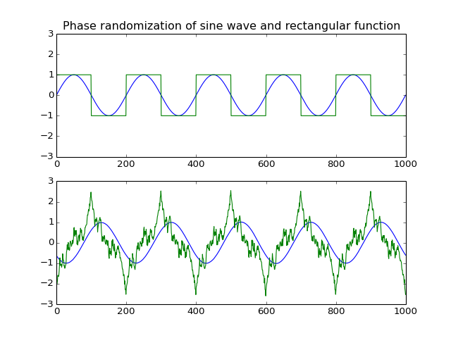
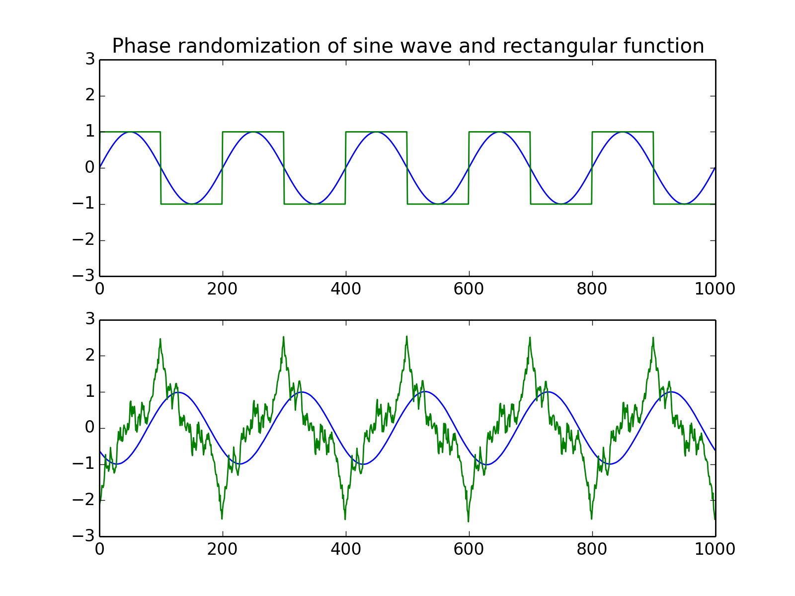
scot.datatools.randomize_phase(data)¶

Phase randomization.

This function randomizes the input array’s spectral phase along the first dimension.

Parameters:

data : array_like

Input array

Returns:

out : ndarray

Array of same shape as data.

Notes

The algorithm randomizes the phase component of the input’s complex fourier transform.

Examples

from pylab import *
from scot.datatools import randomize_phase
np.random.seed(1234)
s = np.sin(np.linspace(0,10*np.pi,1000)).T
x = np.vstack([s, np.sign(s)]).T
y = randomize_phase(x)
subplot(2,1,1)
title('Phase randomization of sine wave and rectangular function')
plot(x), axis([0,1000,-3,3])
subplot(2,1,2)
plot(y), axis([0,1000,-3,3])
plt.show()

(Source code, png, hires.png, pdf)

`matfiles` Module¶

Summary¶

Routines for loading and saving Matlab’s .mat files.

scot.matfiles.loadmat(filename)¶: This function should be called instead of direct spio.loadmat as it cures the problem of not properly recovering python dictionaries from mat files. It calls the function check keys to cure all entries which are still mat-objects

`ooapi` Module¶

Summary¶

Object oriented API to SCoT.

Extended Summary¶

The object oriented API provides a the Workspace class, which provides high-level functionality and serves as an example usage of the low-level API.

class scot.ooapi.Workspace(var, locations=None, reducedim=0.99, nfft=512, fs=2, backend=None)¶

Bases: builtins.object

SCoT Workspace

This class provides high-level functionality for source identification, connectivity estimation, and visualization.

Parameters:

var : {VARBase-like object, dict}

Vector autoregressive model (VAR) object that is used for model fitting. This can also be a dictionary that is passed as **kwargs to backend[‘var’]() in order to construct a new VAR model object.

locations : array_like, optional

3D Electrode locations. Each row holds the x, y, and z coordinates of an electrode.

reducedim : {int, float, ‘no_pca’}, optional

A number of less than 1 in interpreted as the fraction of variance that should remain in the data. All components that describe in total less than 1-reducedim of the variance are removed by the PCA step. An integer numer of 1 or greater is interpreted as the number of components to keep after applying the PCA. If set to ‘no_pca’ the PCA step is skipped.

nfft : int, optional

Number of frequency bins for connectivity estimation.

backend : dict-like, optional

Specify backend to use. When set to None the backend configured in config.backend is used.

Attributes

unmixing_	(array) Estimated unmixing matrix.
mixing_	(array) Estimated mixing matrix.
plot_diagonal	(str) Configures what is plotted in the diagonal subplots. ‘topo’ (default) plots topoplots on the diagonal, ‘S’ plots the spectral density of each component, and ‘fill’ plots connectivity on the diagonal.
plot_outside_topo	(bool) Whether to place topoplots in the left column and top row.
plot_f_range	((int, int)) Lower and upper frequency limits for plotting. Defaults to [0, fs/2].

compare_conditions(labels1, labels2, measure_name, alpha=0.01, repeats=100, num_samples=None, plot=False)¶

Test for significant difference in connectivity of two sets of class labels.

Connectivity estimates are obtained by bootstrapping. Correction for multiple testing is performed by controlling the false discovery rate (FDR).

Parameters:

labels1, labels2 : list of class labels

The two sets of class labels to compare. Each set may contain more than one label.

measure_name : str

Name of the connectivity measure to calculate. See Connectivity for supported measures.

alpha : float, optional

Maximum allowed FDR. The ratio of falsely detected significant differences is guaranteed to be less than alpha.

repeats : int, optional

How many bootstrap estimates to take.

num_samples : int, optional

How many samples to take for each bootstrap estimates. Defaults to the same number of trials as present in the data.

plot : {False, None, Figure object}, optional

Whether and where to plot the connectivity. If set to False, nothing is plotted. Otherwise set to the Figure object. If set to None, a new figure is created.

Returns:

p : array, shape = [n_channels, n_channels, nfft]

Uncorrected p-values.

s : array, dtype=bool, shape = [n_channels, n_channels, nfft]

FDR corrected significance. True means the difference is significant in this location.

fig : Figure object, optional

Instance of the figure in which was plotted. This is only returned if plot is not False.

do_ica()¶

Perform ICA

Perform plain ICA source decomposition.

Returns:

result : class

see plainica() for a description of the return value.

Raises:

RuntimeError

If the Workspace instance does not contain data.

do_mvarica(varfit='ensemble')¶

Perform MVARICA

Perform MVARICA source decomposition and VAR model fitting.

Parameters:

varfit : string

Determines how to calculate the residuals for source decomposition. ‘ensemble’ (default) fits one model to the whole data set, ‘class’ fits a different model for each class, and ‘trial’ fits a different model for each individual trial.

Returns:

result : class

see mvarica() for a description of the return value.

Raises:

RuntimeError

If the Workspace instance does not contain data.

fit_var()¶

Fit a var model to the source activations.

Raises:

RuntimeError

If the Workspace instance does not contain source activations.

get_bootstrap_connectivity(measure_names, repeats=100, num_samples=None, plot=False)¶

Calculate bootstrap estimates of spectral connectivity measures.

Bootstrapping is performed on trial level.

Parameters:

measure_names : {str, list of str}

Name(s) of the connectivity measure(s) to calculate. See Connectivity for supported measures.

repeats : int, optional

How many bootstrap estimates to take.

num_samples : int, optional

How many samples to take for each bootstrap estimates. Defaults to the same number of trials as present in the data.

Returns:

measure : array, shape = [repeats, n_channels, n_channels, nfft]

Values of the connectivity measure for each bootstrap estimate. If measure_names is a list of strings a dictionary is returned, where each key is the name of the measure, and the corresponding values are ndarrays of shape [repeats, n_channels, n_channels, nfft].

See also

scot.connectivity_statistics.bootstrap_connectivity(): Calculates bootstrap connectivity

get_connectivity(measure_name, plot=False)¶

Calculate spectral connectivity measure.

Parameters:

measure_name : str

Name of the connectivity measure to calculate. See Connectivity for supported measures.

plot : {False, None, Figure object}, optional

Whether and where to plot the connectivity. If set to False, nothing is plotted. Otherwise set to the Figure object. If set to None, a new figure is created.

Returns:

measure : array, shape = [n_channels, n_channels, nfft]

Values of the connectivity measure.

fig : Figure object

Instance of the figure in which was plotted. This is only returned if plot is not False.

Raises:

RuntimeError

If the Workspace instance does not contain a fitted VAR model.

get_surrogate_connectivity(measure_name, repeats=100)¶

Calculate spectral connectivity measure under the assumption of no actual connectivity.

Repeatedly samples connectivity from phase-randomized data. This provides estimates of the connectivity distribution if there was no causal structure in the data.

Parameters:

measure_name : str

Name of the connectivity measure to calculate. See Connectivity for supported measures.

repeats : int, optional

How many surrogate samples to take.

Returns:

measure : array, shape = [repeats, n_channels, n_channels, nfft]

Values of the connectivity measure for each surrogate.

Raises:

RuntimeError

If the Workspace instance does not contain a fitted VAR model.

See also

scot.connectivity_statistics.surrogate_connectivity(): Calculates surrogate connectivity

get_tf_connectivity(measure_name, winlen, winstep, plot=False)¶

Calculate estimate of time-varying connectivity.

Connectivity is estimated in a sliding window approach on the current data set. The window is stepped n_steps = (n_samples - winlen) // winstep times.

Parameters:

measure_name : str

Name of the connectivity measure to calculate. See Connectivity for supported measures.

winlen : int

Length of the sliding window (in samples).

winstep : int

Step size for sliding window (in samples).

plot : {False, None, Figure object}, optional

Whether and where to plot the connectivity. If set to False, nothing is plotted. Otherwise set to the Figure object. If set to None, a new figure is created.

Returns:

result : array, shape = [n_channels, n_channels, nfft, n_steps]

Values of the connectivity measure.

fig : Figure object, optional

Instance of the figure in which was plotted. This is only returned if plot is not False.

Raises:

RuntimeError

If the Workspace instance does not contain a fitted VAR model.

optimize_var()¶

Optimize the var model’s hyperparameters (such as regularization).

Raises:

RuntimeError

If the Workspace instance does not contain source activations.

plot_connectivity_surrogate(measure_name, repeats=100, fig=None)¶

Plot spectral connectivity measure under the assumption of no actual connectivity.

Repeatedly samples connectivity from phase-randomized data. This provides estimates of the connectivity distribution if there was no causal structure in the data.

Parameters:

measure_name : str

Name of the connectivity measure to calculate. See Connectivity for supported measures.

repeats : int, optional

How many surrogate samples to take.

fig : {None, Figure object}, optional

Where to plot the topos. f set to None, a new figure is created. Otherwise plot into the provided figure object.

Returns:

fig : Figure object

Instance of the figure in which was plotted.

plot_connectivity_topos(fig=None)¶

Plot scalp projections of the sources.

This function only plots the topos. Use in combination with connectivity plotting.

Parameters:

fig : {None, Figure object}, optional

Where to plot the topos. f set to None, a new figure is created. Otherwise plot into the provided figure object.

Returns:

fig : Figure object

Instance of the figure in which was plotted.

plot_source_topos(common_scale=None)¶

Plot topography of the Source decomposition.

Parameters:

common_scale : float, optional

If set to None, each topoplot’s color axis is scaled individually. Otherwise specifies the percentile (1-99) of values in all plot. This value is taken as the maximum color scale.

remove_sources(sources)¶

Remove sources from the decomposition.

This function removes sources from the decomposition. Doing so invalidates currently fitted VAR models and connectivity estimates.

Parameters:

sources : {slice, int, array of ints}

Indices of components to remove.

Raises:

RuntimeError

If the Workspace instance does not contain a source decomposition.

set_data(data, cl=None, time_offset=0)¶

Assign data to the workspace.

This function assigns a new data set to the workspace. Doing so invalidates currently fitted VAR models, connectivity estimates, and activations.

Parameters:

data : array-like, shape = [n_samples, n_channels, n_trials] or [n_samples, n_channels]

EEG data set

cl : list of valid dict keys

Class labels associated with each trial.

time_offset : float, optional

Trial starting time; used for labelling the x-axis of time/frequency plots.

set_used_labels(labels)¶

Specify which trials to use in subsequent analysis steps.

This function masks trials based on their class labels.

Parameters:

labels : list of class labels

Marks all trials that have a label that is in the labels list for further processing.

static show_plots()¶

Show current plots.

This is only a convenience wrapper around matplotlib.pyplot.show_plots().

`plainica` Module¶

Source decomposition with ICA.

class scot.plainica.ResultICA(mx, ux)¶

Bases: builtins.object

Result of plainica()

Attributes

mixing	(array) estimate of the mixing matrix
unmixing	(array) estimate of the unmixing matrix

scot.plainica.plainica(x, reducedim=0.99, backend=None)¶

Source decomposition with ICA.

Apply ICA to the data x, with optional PCA dimensionality reduction.

Parameters:

x : array-like, shape = [n_samples, n_channels, n_trials] or [n_samples, n_channels]

data set

reducedim : {int, float, ‘no_pca’}, optional

A number of less than 1 in interpreted as the fraction of variance that should remain in the data. All components that describe in total less than 1-reducedim of the variance are removed by the PCA step. An integer numer of 1 or greater is interpreted as the number of components to keep after applying the PCA. If set to ‘no_pca’ the PCA step is skipped.

backend : dict-like, optional

Specify backend to use. When set to None the backend configured in config.backend is used.

Returns:

result : ResultICA

Source decomposition

`plotting` Module¶

Graphical output with matplotlib

This module attempts to import matplotlib for plotting functionality. If matplotlib is not available no error is raised, but plotting functions will not be available.

scot.plotting.plot_circular(widths, colors, curviness=0.2, mask=True, topo=None, topomaps=None, axes=None, order=None)¶

Circluar connectivity plot

Topos are arranged in a circle, with arrows indicating connectivity

Parameters:

widths : {float or array, shape = [n_channels, n_channels]}

Width of each arrow. Can be a scalar to assign the same width to all arrows.

colors : array, shape = [n_channels, n_channels, 3] or [3]

RGB color values for each arrow or one RGB color value for all arrows.

curviness : float, optional

Factor that determines how much arrows tend to deviate from a straight line.

mask : array, dtype = bool, shape = [n_channels, n_channels]

Enable or disable individual arrows

topo : Topoplot

This object draws the topo plot

topomaps : array, shape = [w_pixels, h_pixels]

Scalp-projected map

axes : axis, optional

Axis to draw into. A new figure is created by default.

order : list of int

Rearrange channels.

Returns:

fig : Figure object

The figure into which was plotted.

scot.plotting.plot_connectivity_significance(s, fs=2, freq_range=(-inf, inf), diagonal=0, border=False, fig=None)¶

Plot significance.

Significance is drawn as a background image where dark vertical stripes indicate freuquencies where a evaluates to True.

Parameters:

a : array, dtype=bool, shape = [n_channels, n_channels, n_fft]

Significance

fs : float

Sampling frequency

freq_range : (float, float)

Frequency range to plot

diagonal : {-1, 0, 1}

If diagonal == -1 nothing is plotted on the diagonal (a[i,i,:] are not plotted), if diagonal == 0, a is plotted on the diagonal too (all a[i,i,:] are plotted), if diagonal == 1, a is plotted on the diagonal only (only a[i,i,:] are plotted)

border : bool

If border == true the leftmost column and the topmost row are left blank

fig : Figure object, optional

Figure to plot into. If set to None, a new figure is created.

Returns:

fig : Figure object

The figure into which was plotted.

scot.plotting.plot_connectivity_spectrum(a, fs=2, freq_range=(-inf, inf), diagonal=0, border=False, fig=None)¶

Draw connectivity plots.

Parameters:

a : array, shape = [n_channels, n_channels, n_fft] or [1 or 3, n_channels, n_channels, n_fft]

If a.ndim == 3, normal plots are created, If a.ndim == 4 and a.shape[0] == 1, the area between the curve and y=0 is filled transparently, If a.ndim == 4 and a.shape[0] == 3, a[0,:,:,:] is plotted normally and the area between a[1,:,:,:] and a[2,:,:,:] is filled transparently.

fs : float

Sampling frequency

freq_range : (float, float)

Frequency range to plot

diagonal : {-1, 0, 1}

If diagonal == -1 nothing is plotted on the diagonal (a[i,i,:] are not plotted), if diagonal == 0, a is plotted on the diagonal too (all a[i,i,:] are plotted), if diagonal == 1, a is plotted on the diagonal only (only a[i,i,:] are plotted)

border : bool

If border == true the leftmost column and the topmost row are left blank

fig : Figure object, optional

Figure to plot into. If set to None, a new figure is created.

Returns:

fig : Figure object

The figure into which was plotted.

scot.plotting.plot_connectivity_timespectrum(a, fs=2, crange=None, freq_range=(-inf, inf), time_range=None, diagonal=0, border=False, fig=None)¶

Draw time/frequency connectivity plots.

Parameters:

a : array, shape = [n_channels, n_channels, n_fft, n_timesteps]

Values to draw

fs : float

Sampling frequency

crange : [int, int], optional

Range of values covered by the colormap. If set to None, [min(a), max(a)] is substituted.

freq_range : (float, float)

Frequency range to plot

time_range : (float, float)

Time range covered by a

diagonal : {-1, 0, 1}

If diagonal == -1 nothing is plotted on the diagonal (a[i,i,:] are not plotted), if diagonal == 0, a is plotted on the diagonal too (all a[i,i,:] are plotted), if diagonal == 1, a is plotted on the diagonal only (only a[i,i,:] are plotted)

border : bool

If border == true the leftmost column and the topmost row are left blank

fig : Figure object, optional

Figure to plot into. If set to None, a new figure is created.

Returns:

fig : Figure object

The figure into which was plotted.

scot.plotting.plot_connectivity_topos(layout='diagonal', topo=None, topomaps=None, fig=None)¶

Place topo plots in a figure suitable for connectivity visualization.

Note

Parameter topo is modified by the function by calling set_map().

Parameters:

layout : str

‘diagonal’ -> place topo plots on diagonal. otherwise -> place topo plots in left column and top row.

topo : Topoplot

This object draws the topo plot

topomaps : array, shape = [w_pixels, h_pixels]

Scalp-projected map

fig : Figure object, optional

Figure to plot into. If set to None, a new figure is created.

Returns:

fig : Figure object

The figure into which was plotted.

scot.plotting.plot_sources(topo, mixmaps, unmixmaps, global_scale=None, fig=None)¶

Plot all scalp projections of mixing- and unmixing-maps.

Note

Parameter topo is modified by the function by calling set_map().

Parameters:

topo : Topoplot

This object draws the topo plot

mixmaps : array, shape = [w_pixels, h_pixels]

Scalp-projected mixing matrix

unmixmaps : array, shape = [w_pixels, h_pixels]

Scalp-projected unmixing matrix

global_scale : float, optional

Set common color scale as given percentile of all map values to use as the maximum. None scales each plot individually (default).

fig : Figure object, optional

Figure to plot into. If set to None, a new figure is created.

Returns:

fig : Figure object

The figure into which was plotted.

scot.plotting.plot_topo(axis, topo, topomap, crange=None, offset=(0, 0))¶

Draw a topoplot in given axis.

Note

Parameter topo is modified by the function by calling set_map().

Parameters:

axis : axis

Axis to draw into.

topo : Topoplot

This object draws the topo plot

topomap : array, shape = [w_pixels, h_pixels]

Scalp-projected data

crange : [int, int], optional

Range of values covered by the colormap. If set to None, [-max(abs(topomap)), max(abs(topomap))] is substituted.

offset : [float, float], optional

Shift the topo plot by [x,y] in axis units.

Returns:

h : image

Image object the map was plotted into

scot.plotting.plot_whiteness(var, h, repeats=1000, axis=None)¶

Draw distribution of the Portmanteu whiteness test.

Parameters:

var : VARBase-like object

Vector autoregressive model (VAR) object whose residuals are tested for whiteness.

h : int

Maximum lag to include in the test.

repeats : int, optional

Number of surrogate estimates to draw under the null hypothesis.

axis : axis, optional

Axis to draw into. By default draws into matplotlib.pyplot.gca().

Returns:

pr : float

p-value of whiteness under the null hypothesis

scot.plotting.prepare_topoplots(topo, values)¶

Prepare multiple topo maps for cached plotting.

Note

Parameter topo is modified by the function by calling set_values().

Parameters:

topo : Topoplot

Scalp maps are created with this class

values : array, shape = [n_topos, n_channels]

Channel values for each topo plot

Returns:

topomaps : list of array

The map for each topo plot

scot.plotting.show_plots()¶

`utils` Module¶

Utility functions

class scot.utils.DocStringInheritor¶

Bases: builtins.object

The most base type

class scot.utils.DocStringInheritorMeta¶

Bases: builtins.type

Inherit doc strings from base class.

Based on unutbu’s DocStringInheritor [R4] which is a variation of Paul McGuire’s DocStringInheritor [R5]

References

[R4]	(1, 2) http://stackoverflow.com/a/8101118

[R5]	(1, 2) http://groups.google.com/group/comp.lang.python/msg/26f7b4fcb4d66c95

scot.utils.acm(x, l)¶

Autocovariance matrix at lag l

This function calculates the autocovariance matrix of x at lag l.

Parameters:

x : ndarray, shape = [n_samples, n_channels, (n_trials)]

Signal data (2D or 3D for multiple trials)

l : int

Lag

Returns:

c : ndarray, shape = [nchannels, n_channels]

Autocovariance matrix of x at lag l.

scot.utils.cuthill_mckee(matrix)¶

Cuthill-McKee algorithm

Permute a symmetric binary matrix into a band matrix form with a small bandwidth.

Parameters:

matrix : ndarray, dtype=bool, shape = [n, n]

The matrix is internally converted to a symmetric matrix by setting each element [i,j] to True if either [i,j] or [j,i] evaluates to true.

Returns:

order : list of int

Permutation intices

class scot.utils.memoize(func)¶

Bases: builtins.object

cache the return value of a method

This class is meant to be used as a decorator of methods. The return value from a given method invocation will be cached on the instance whose method was invoked. All arguments passed to a method decorated with memoize must be hashable.

If a memoized method is invoked directly on its class the result will not be cached. Instead the method will be invoked like a static method: class Obj(object):

@memoize def add_to(self, arg):

return self + arg

Obj.add_to(1) # not enough arguments Obj.add_to(1, 2) # returns 3, result is not cached

`var` Module¶

vector autoregressive (VAR) model

class scot.var.Defaults¶

Bases: builtins.object

xvschema(t, num_trials)¶: Multi-trial cross-validation schema: use one trial for testing, all others for training.

class scot.var.VARBase(model_order)¶

Bases: scot.utils.DocStringInheritor

Represents a vector autoregressive (VAR) model.

Note on the arrangement of model coefficients:

b is of shape m, m*p, with sub matrices arranged as follows:: b_00 b_01 ... b_0m b_10 b_11 ... b_1m .... .... .... b_m0 b_m1 ... b_mm

Each sub matrix b_ij is a column vector of length p that contains the filter coefficients from channel j (source) to channel i (sink).

copy()¶

fit(data)¶: Fit the model to data.

is_stable()¶: Test if the VAR model is stable.

optimize(data)¶: Optimize the var model’s hyperparameters (such as regularization).

predict(data)¶

Predict samples from actual data.

Note that the model requires p past samples for prediction. Thus, the first p samples are invalid and set to 0, where p is the model order.

simulate(l, noisefunc=None)¶: Simulate vector autoregressive (VAR) model with optional noise generating function.

test_whiteness(h, repeats=100, get_q=False)¶

Test if the VAR model residuals are white (uncorrelated up to a lag of h).

This function calculates the Li-McLeod as Portmanteau test statistic Q to test against the null hypothesis H0: “the residuals are white” [1]. Surrogate data for H0 is created by sampling from random permutations of the residuals.

Usually the returned p-value is compared against a pre-defined type 1 error level of alpha=0.05 or alpha=0.01. If p<=alpha, the hypothesis of white residuals is rejected, which indicates that the VAR model does not properly describe the data.

scot.var.fit_multiclass(data, cl, p ) fit_multiclass( data, cl, p, delta)¶

Fits a separate autoregressive model for each class.

If sqrtdelta is provited and nonzero, the least squares estimation is regularized with ridge regression.

scot.var.test_whiteness(data, h, p=0, repeats=100, get_q=False)¶

Test if signals are white (uncorrelated up to a lag of h).

This function calculates the Li-McLeod as Portmanteau test statistic Q to test against the null hypothesis H0: “the signals are white” [1]. Surrogate data for H0 is created by sampling from random permutations of the signals.

Usually the returned p-value is compared against a pre-defined type 1 error level of alpha=0.05 or alpha=0.01. If p<=alpha, the hypothesis of white signals is rejected.

`varica` Module¶

scot.varica.mvarica(x, p ) mvarica( x, p, retain_variance, delta ) mvarica( x, p, numcomp, delta)¶

Apply MVARICA to the data x. MVARICA performs the following steps:

Optional dimensionality reduction with PCA
Fitting a VAR model tho the data
Decomposing the VAR model residuals with ICA
Correcting the VAR coefficients

`xvschema` Module¶

Cross-validation schemas

scot.xvschema.multitrial(t, num_trials)¶: Multi-trial cross-validation schema: use one trial for testing, all others for training.

scot.xvschema.singletrial(t, num_trials)¶: Single-trial cross-validation schema: use one trial for training, all others for testing.

Table Of Contents

Previous topic

Next topic

This Page

scot Package¶

`scot` Package¶

`config` Module¶

`connectivity` Module¶

`connectivity_statistics` Module¶

`datatools` Module¶

Summary¶

`matfiles` Module¶

Summary¶

`ooapi` Module¶

Summary¶

Extended Summary¶

`plainica` Module¶

`plotting` Module¶

`utils` Module¶

`var` Module¶

`varica` Module¶

`xvschema` Module¶

Subpackages¶

Navigation

Table Of Contents

Previous topic

Next topic

This Page

Quick search

scot Package¶

scot Package¶

config Module¶

connectivity Module¶

connectivity_statistics Module¶

datatools Module¶

Summary¶

matfiles Module¶

Summary¶

ooapi Module¶

Summary¶

Extended Summary¶

plainica Module¶

plotting Module¶

utils Module¶

var Module¶

varica Module¶

xvschema Module¶

Subpackages¶

Navigation

`scot` Package¶

`config` Module¶

`connectivity` Module¶

`connectivity_statistics` Module¶

`datatools` Module¶

`matfiles` Module¶

`ooapi` Module¶

`plainica` Module¶

`plotting` Module¶

`utils` Module¶

`var` Module¶

`varica` Module¶

`xvschema` Module¶